Generative Relations in Legal Judgment - Evidence, Historical Trajectories, and Norm-Relevant Similarity
Transcript
Abstract
Legal comparison depends on the relationship between general norms and particular histories. Identical words or recorded outcomes can arise through different dependencies, while different expressions can perform comparable functions within a relationship. This discussion paper develops an account of norm-relevant similarity through the reconstruction of generative relations: the processes through which resources, expectations, interpretations, and available actions become connected over time. It distinguishes evidential support, causal reconstruction, normative characterization, and institutional authority. A fictional reimbursement rule and a controlled family of cases make the comparison criteria explicit without asserting current doctrine. A relational-field formulation then separates observation from retained history and counterfactual response, while requiring role-preserving mappings, justified time scales, and independently defended normative constraints. Completed synthetic calculations show how shared trajectories, attractors, action values, or boundary amplitudes can coexist with differences in dynamics or interior histories. These results supply mathematical examples of limited inference; they provide no empirical validation of legal decision-making. The paper grounds reason-giving, contestation, and proportionate correction in stated commitments to equal standing, protection against material error, and accountable public authority. Its contribution is an inspectable connection between historical reconstruction and issue-specific comparison, with established legal analogy and case-based reasoning as substantive baselines.
Keywords: legal judgment; evidence; relational history; legal analogy; norm-relevant similarity; interpretive correction.
Research Paper Note
This legal-philosophical discussion paper develops a framework for evidential reconstruction and norm-relevant comparison. Its rule and cases are fictional. The mathematical studies establish properties of stipulated models and have not been validated against actual legal judgments.
The project welcomes objections, corrections, and identification of related concepts in other disciplines. It claims no priority in legal analogy, context-sensitive reasoning, interpretive justice, procedural correction, or dynamical approaches to social relations. Relevant antecedents include research on forensic relevance, legal analogy, case-based legal reasoning, and attraction basins for generative justice (Gardner et al. 2019; Lamond 2014; Ashley 1992; Ashley and Rissland 2003; Eglash and Garvey 2014). The proposed Generative Relational vocabulary requires comparison with these traditions. Access limitations and remaining reading are stated in the source ledger.
Responsible Use and Rights Reservation
This section records requested scholarly conduct and the scope of retained rights. The scholarly requests accompany the preprint licence and create no additional condition on permissions granted by that licence.
Good-faith criticism, correction, and independent development are welcome. Relational reconstructions should retain their supporting evidence, counterevidence, uncertainty, and normative scope. Model outputs should remain identified as consequences of stated assumptions. Institutional use requires an argument about authority and affected interests in addition to any formal analysis.
Rights outside the preprint licence remain with their respective holders. Ethical requests create no additional licence condition. No exclusive entitlement to the concepts, mathematical tools, or independent formulations discussed in the paper is asserted.
Notices
Preprint status.
This is a discussion preprint. Independent human peer review has not been completed. The arguments, interpretations, and proposed applications remain open to correction.
Preprint licence.
The original material in this preprint is made available under Creative Commons Attribution–NonCommercial 4.0 International (CC BY-NC 4.0), https://creativecommons.org/licenses/by-nc/4.0/, to the extent that copyright or related rights apply and are held by the contributors. Reuse should follow the licence’s attribution and noncommercial conditions, retain the licence notice, and identify changes. Separately identified third-party material retains its own rights and permissions. Material in the public domain and uses permitted by applicable exceptions remain unaffected. The official licence controls its terms.
AI-use disclosure.
The supplied exploratory human–AI conversation informed the research questions. An OpenAI coding assistant prepared the outline, initial source checks, methodological criticisms, a proposed relational-field formulation, an executable synthetic illustration, the complete first manuscript draft, and the expanded preprint revision. AI assistance involved substantive argument, analysis, and writing, beyond language editing or formatting. The illustration concerns a constructed transition system and supplies no independent empirical validation of the proposed account. A companion Paper I pilot collected 24 actual agent responses about reality attribution, and a separate spatial field experiment was run in Python. Neither evaluates legal interpretation or validates judicial performance. No such validation follows from the subsequent field-equivalence, action, and finite-group boundary calculations either. Their analytic and numerical comparisons concern specified synthetic structures. No legal-response experiment or expert study has been conducted.
Human attribution.
The author is Wanhong HUANG, contact huangwanhong@serendip.ngo. AI systems are disclosed as research and drafting tools. The author attribution identifies the human contributor and does not represent independent peer review. Earlier sources and PDFs are preserved in the project version archive.
Introduction
This paper examines how legal judgment can compare particular histories while remaining accountable to general norms. Its purpose is to clarify the relation among evidential reconstruction, causal explanation, the selection of relevant similarities, and the authority of a conclusion. The discussion develops a fictional rule and a family of controlled cases, then uses finite transition systems and field-based mathematical examples to expose limits of compressed comparison. The resulting proposal concerns the organization and criticism of reasons; it is a discussion framework without validation against actual judicial decisions.
Two cases can end in the same recorded event and differ in the path by which that event became possible. A person may accept an arrangement after an ordinary offer, after a threat affecting access to an essential resource, or after the removal of a constraint that previously limited choice. If a legal issue concerns coercion, dependence, or the practical availability of refusal, a terminal description can omit a distinction selected by the norm. Yet the inclusion of a richer history cannot itself establish its legal significance. An investigator must support the history with evidence and explain the rule under which the difference matters.
These obligations arise at different stages. A report is evidence about an event; a causal account proposes how events are connected; a comparison selects features shared across histories; and a judgment applies an institutionally situated standard. Errors occur when one stage silently substitutes for another. A coherent narrative can remain evidentially weak. A reliable prediction can depend on features with doubtful relevance to the issue. A close mathematical match can erase the roles or temporal conditions that make a legal distinction intelligible. The paper develops a way to keep these obligations visible within a connected account.
The phrase generative relations emphasizes the processes through which positions, opportunities, constraints, and responses develop. The proposed unit of comparison includes the history relevant to a stated issue, with explicit attention to the people and resources whose relations the norm selects. This emphasis has antecedents in legal analogy, case-based reasoning, causal inquiry, epistemic injustice, and relational accounts of justice. The paper claims no priority over those traditions. Its contribution is a structured discussion of their intersection with the distinct meanings of similarity and equivalence in mathematical models.
The fictional Rule R makes the inferential stages inspectable without presenting an invented rule as law in any jurisdiction. Its case family holds some descriptions fixed while varying a prior threat, a refusal path, a resource floor, and evidence of the relevant relation. A finite enumeration verifies consequences within stipulated transitions. The field examples then show how equal outputs, oriented trajectories, asymptotic states, action values, or boundary amplitudes can preserve different information. These mathematical results establish limitations of particular inference patterns. The normative importance of the lost information remains a matter for the defended rule, evidence, and institutional context.
Section 2 reviews the relevant antecedents. Sections 3 onward develop the evidential problem and the fictional cases before specifying norm-relevant comparison. The later sections examine field models, actions and boundary descriptions, public correction, and objections. Section 12 states the proposed institutional research agenda. The appendices integrate the complete finite comparison, restrictions on comparison maps, and shared mathematical studies into this paper. The companion paper, Human and Artificial Reality: Generative Relations and the Formation of Interpretation, addresses the philosophical problem of reality attribution and contains the live-agent response corpus. That pilot supplies no empirical legal validation for the present proposal.
Literature Review
This section identifies antecedents for the paper’s treatment of norms, analogy, evidence, causal reconstruction, justice, and mathematical comparison. The review is selective and organized by argumentative role. It makes no claim to exhaust the jurisprudential literature or to settle differences among its traditions. Sources were verified online before citation; attributions remain within the abstract, metadata, or original passages actually consulted. The purpose is to locate the proposed framework and identify the work required for a more complete doctrinal and empirical assessment.
Norms, Principles, and the Structure of Reasons
Dworkin’s The Model of Rules is a foundational point of reference for the structure of legal reasons. In the inspected discussion, principles possess a dimension of weight or importance, whose assessment can be controversial and does not constitute exact measurement (Dworkin 1967). This distinction is relevant to the temptation to turn every normative consideration into a numerical coefficient. A model that aggregates features needs an independent account of the kind of reason each feature supplies and the permissibility of compensation among them.
The present use of Rule R has a more limited methodological purpose. A stipulated rule exposes how a conclusion depends on specified conditions. It does not imply that actual legal practice consists entirely of such rules, or that contested principles can always be reduced to a Boolean checklist. The fictional construction holds normative conditions sufficiently stable to examine evidential and temporal differences. Extension to a real controversy would require an account of legal authority, interpretation, exceptions, burdens of proof, and the relations among potentially competing reasons.
This separation preserves an important place for disagreement. Participants may agree about events and disagree about the rule, agree about the rule and disagree about the evidence, or share both while disputing whether a case falls within an exception. A useful decision record should show which dispute remains. Increasing the detail of a field model cannot resolve an unsettled issue of authority merely through greater mathematical precision.
Relational Analogy and Legal Case Comparison
Gentner’s structure-mapping account of analogy distinguishes relational mapping from a comparison based only on attributes and gives higher-order systematicity a central role (Gentner 1983). This is an antecedent for examining patterns of relations across cases. A mapping between a resource controller, a dependent participant, an available refusal, and an anticipated consequence can preserve information that a list of endpoint attributes omits. The normative permission to use such a mapping remains separate from its descriptive coherence.
Legal analogy has its own established analyses. Lamond distinguishes forms of analogical reasoning in common-law practice, including classificatory, close, and distant analogies (Lamond 2014). Ashley’s work places legal case-based reasoning within a developed computational tradition, and Ashley and Rissland examine law, learning, and representation (Ashley 1992; Ashley and Rissland 2003). These sources rule out a novelty claim based merely on comparing cases, encoding distinctions, or attending to representation. The present proposal concerns the explicit temporal and normative conditions under which a relation preserved by a model can support a particular legal comparison.
The distinction between retrieval and justification follows from this positioning. Similarity can help locate cases for inspection. A selected case then requires explanation of the respects in which it bears on the issue. An algorithm may give a close match because many observable details agree while omitting the role relation that controls the legal question. Conversely, cases that differ in ordinary descriptive distance can share the structure selected by a norm. The discussion below treats a similarity measure as one possible instrument within a reason-giving process, with the selection and interpretation of its features available for criticism.
Evidence, Relevance, and Counterfactual Reconstruction
Research on forensic decision making already investigates the relevance of contextual information. Gardner and colleagues’ study of forensic analysts addresses which information practitioners consider relevant to their decisions (Gardner et al. 2019). The present argument should therefore be read as a further specification of relevance under a selected issue. It does not portray legal or forensic inquiry as uniformly indifferent to context.
Pearl’s overview of causal inference emphasizes the assumptions required for causal and counterfactual claims and distinguishes queries about interventions, counterfactuals, and related effects (Pearl 2009). This antecedent clarifies the status of a reconstructed refusal path. Observed acceptance under one set of conditions does not, by itself, identify the result of a different intervention. A causal interpretation combines evidence with assumptions about the relevant response mechanism. The paper’s transition model makes those assumptions explicit, allowing their consequences to be checked while leaving their real-world adequacy unresolved.
The evidential problem is especially acute when the allegedly constrained option was never attempted. A counterfactual refusal can be supported by prior communications, control over resources, observed responses to similar refusals, and evidence about feasible alternatives. Each item has a provenance and a possible competing interpretation. A field representation can organize a proposed account of these relations, but the diagram or trajectory does not add an observation merely by displaying it. The case analysis therefore distinguishes recorded events, supported inferences, stipulated assumptions, and unresolved alternatives.
The framework also separates causal and normative thresholds. A causal contribution to an outcome can exist without satisfying the conditions of a particular legal wrong. Conversely, a norm can make a threatened consequence relevant even when a later intervention prevents that consequence from occurring. The appropriate comparison depends on what the rule selects, when it selects it, and what the evidence can establish about the affected person’s situation.
Interpretive Resources and Epistemic Injustice
Fricker’s treatment of hermeneutical injustice concerns disadvantages associated with the resources available for making experience intelligible (Fricker 2007). Flores’s discussion of trauma and elite capture supplies a further examination of the politics of interpretive categories (Flores 2025). These antecedents motivate attention to whose descriptions enter a record and whose experience can be articulated through the categories an institution accepts.
The present framework treats these concerns as reasons to inspect the production of evidence as well as its final form. A missing category, an inaccessible procedure, or an asymmetric opportunity to explain a history can affect what later appears in a dataset. Enlarging a feature vector cannot automatically recover information that was never recorded or that was systematically excluded. Attention to historical relations should therefore include the history of the record itself: its collection, compression, classification, and revision.
This commitment also limits inference from fluent articulation. A coherent and institutionally familiar account can receive attention unavailable to an awkward or unfamiliar one. Neither fluency nor difficulty establishes truth by itself. The proposed decision record should retain reasons for accepting or rejecting a claim and make it possible to challenge the categories through which the claim was understood. These requirements concern evidential accountability; they leave the substantive resolution of a disputed case to its supported facts and governing norms.
Generative Justice, Public Deliberation, and Revision
Eglash and Garvey’s discussion of basins of attraction and generative justice is a direct antecedent for bringing dynamical language into a discussion of justice (Eglash and Garvey 2014). Both authors and the existing concept must be acknowledged. The present paper uses generative relations to organize a question about legal histories and comparison; it does not claim to originate generative justice or to reproduce that chapter’s full program.
Niemeyer and Dryzek’s account of meta-consensus provides an antecedent for examining common commitments amid continuing substantive disagreement (Niemeyer and Dryzek 2007). Nobles and Schiff locate legal pluralism within a systems-theoretic discussion (Nobles and Schiff 2012). These references help frame the institutional problem of publicly defensible comparison across differences in interpretation. They do not supply a theorem guaranteeing convergence or agreement in the proposed procedure.
Revision also has a specific literature. Tutt’s revisability principle concerns a narrower problem involving identity and records (Tutt 2015); it should not be treated as a general theory of judicial appeal. The extension pursued here is expressly argumentative: where a judgment relies on an evidential or interpretive compression, a later challenge should be able to identify the material assumption and explain the consequence of revising it. Questions of finality, cost, reliance, and institutional competence remain part of that assessment.
Dynamical and Variational Comparison
Behavioural systems theory and approximation metrics provide mathematical antecedents for distinguishing a representation from its accessible behaviour and for specifying an approximate comparison (Willems 1991; Girard and Pappas 2007). Viability theory supplies an established setting for studying trajectories subject to constraints (Aubin et al. 2011). The finite resource-floor example in this paper is elementary and fully enumerated; it claims no general viability result and no empirical identification of a legally appropriate floor.
Action-based comparison introduces additional structure. Gradient-flow and large-deviation accounts make clear that a functional is interpreted together with dynamics, dissipation, or probabilistic assumptions (Peletier 2014; Adams et al. 2012; Onsager and Machlup 1953). The worked examples below use fixed finite coefficients to distinguish shared energy, different mobilities, pathwise action values, and consistent coordinate transformations. Equality of a scalar evaluated on a path discards information about the path. Whether that discarded information matters legally depends on the issue under consideration.
Spin-foam research and coarse-graining methods provide an established context for boundary amplitudes and consistency across descriptions (Perez 2013; Bahr et al. 2013; Dittrich et al. 2012; Bahr 2014). The present finite-group construction uses positive weights and a directly verifiable dual expansion. It identifies a precise example in which the selected boundary data agree and interior insertions differ. The comparison serves as a mathematical illustration of information retained by a boundary description. It supplies neither a physical theory of law nor a probabilistic model fitted to legal outcomes.
Contribution and Remaining Research
The proposed contribution is a connected discipline of comparison: identify the legal issue and its authority, reconstruct the relevant history from evidence, state the correspondence permitted between cases, and disclose the distinctions a representation removes. The fictional cases and mathematical appendices make selected failures of inference inspectable. They also identify where further work belongs: doctrinal interpretation, evidence about actual decision practices, defensible measurement, and evaluation by affected participants and legal specialists.
This positioning leaves the paper open to correction by established theories and by more economical formulations. A successful relational framework should improve the clarity of reasons and counterarguments in a case. The adoption of a field, action, or state-sum formalism has value only when its defined structures contribute to that task and its assumptions can be defended.
General Norms and Particular Histories in Adjudication
This paper examines how a general norm becomes applicable to a particular history and how that application supports comparison across cases. Its method combines conceptual analysis, a controlled fictional case family, and limited mathematical illustrations. The central proposal is that norm-relevant similarity can depend on the processes through which resources, expectations, interpretations, and available actions became connected over time. The paper calls these productive historical connections generative relations.
Consider a supervisor’s message, “You know what you need to do,” followed by an employee’s signed waiver of reimbursement. The message and signature may be authentic. Their authenticity leaves further questions concerning the message’s understood significance, the employee’s available alternatives, the supervisor’s capacity to impose consequences, and the conditions under which the waiver acquired legal effect. A history of sanctions could make the words operate as a reminder of a credible threat. A history of independent planning could support a different account. The same record fragment can enter competing reconstructions.
The legal issue adds another layer. A rule concerning formal authorization can select different features from a rule concerning induced waiver. Even a well-supported causal account does not determine which rule governs, how a burden of proof operates, or which remedy follows. Legal judgment joins evidential and explanatory tasks with a claim of institutional authority. Its reasons should make the transition among those tasks available for assessment.
Existing legal reasoning already gives substantial attention to context and comparison. Lamond examines forms of analogy in common-law reasoning (Lamond 2014). Ashley’s work on case-based legal systems and Ashley and Rissland’s later treatment of law, learning, and representation provide substantive antecedents for structured case comparison (Ashley 1992; Ashley and Rissland 2003). The proposed framework should be assessed against such approaches in their strongest forms. A representation that already captures temporal order, dependence, and competing reasons may accomplish much of the work described here.
The paper’s proposed contribution is therefore connective and diagnostic. It brings together the reconstruction of a history, the distinction between actual and counterfactual possibilities, the selection of norm-relevant features, and the institutional conditions for correcting an interpretation. Field models make some dependencies explicit, especially when retained states and reciprocal effects matter. Their mathematical vocabulary earns a place only when it clarifies an inferential step or exposes a loss of relevant information.
The normative argument relies on stated premises. A decision-making institution that claims authority over affected persons should recognize their equal standing as participants in the justification of that authority, protect them against material errors within the institution’s remit, and give reasons connecting its coercive or distributive decisions to authorized norms and supported facts. These are commitments defended as part of the proposal. They do not follow from the stability of a social system or the existence of a relational field.
The discussion remains jurisprudential and jurisdiction-neutral. Section 6 defines a fictional workplace rule so that the case comparisons have a determinate issue and burden. The resulting outcomes are consequences of those stipulations. They establish no current legal entitlement and should not be transferred to doctrines of criminal duress, coercive control, complicity, or contract validity without a separate analysis of applicable authority. This restriction gives the example a clear scope while preserving its relevance to the more general problem of norm-guided reconstruction.
Evidence and the Reconstruction of Relational Histories
This section separates the evidential stages through which a record supports a claim about a relationship. It considers provenance, rival histories, causal interpretation, and normative characterization in sequence. The sequence is analytical; actual investigation may move repeatedly between stages as new evidence changes the questions worth asking.
Provenance concerns the relation between an item and the event it purports to record. A message archive may accurately preserve words while omitting earlier communications. A witness may accurately recall a consequence while being mistaken about its cause. Establishing authenticity reduces one kind of uncertainty. It leaves questions of completeness, selection, and interpretation for further inquiry. An investigator should avoid treating the verified existence of a record as verification of every inference attached to it.
A relational history assembles supported events into a temporally ordered account. In the running example, relevant events might include instructions, refusals, changes in access to work, explanations of those changes, and opportunities to obtain assistance. Their significance depends partly on order. A sanction announced after a waiver can influence later conduct; it cannot, solely by occurring later, establish that the employee anticipated it earlier. Evidence of a pre-existing policy could support anticipation, but that would be an additional evidential route.
The reconstruction should retain rival explanations. A reduction in work after refusal might have resulted from retaliation, ordinary scheduling, or an independent change in demand. Temporal succession alone leaves these alternatives available. Evidence that a supervisor explicitly connected the reduction to refusal would bear differently on the alternatives from an unexplained coincidence. The aim is to identify which facts discriminate between accounts, how strongly they do so, and where the record remains inconclusive.
Generative explanation adds a mechanism: an account of how a relationship made a particular event possible or likely. The supervisor’s control over assignments could make a warning credible; the employee’s dependence on those assignments could make refusal costly; repeated sanctions could make an ambiguous expression intelligible as a threat. Each link is a candidate claim requiring support. A coherent narrative can organize evidence without acquiring the evidential status of the facts it organizes.
Counterfactual claims require particular care. An employee’s acceptance does not directly show what would have followed refusal. A mechanism can be supported by previous refusals, explicit policies, contemporaneous statements, or other appropriately relevant evidence. General information about a group may suggest an investigative question, yet the individual attribution needs a warranted connection to the person’s circumstances. The difference between a physically possible action and a practically accessible alternative can be central, but neither should be inferred from group membership alone.
A legal characterization then asks which supported features satisfy the authorized rule. A rule may require a prior threat, a causal contribution, and the absence of a protected alternative. Another may attach consequences to a formal notice regardless of some causal details. The characterization must preserve the difference between an unresolved factual premise and a disagreement about the norm’s meaning. Otherwise, an interpretive dispute can appear to be a factual finding, or an evidential gap can disappear into a broad description of the relationship.
The resulting account of evidence is relational in a precise sense. A record bears on a history through its provenance and content; a history supports a mechanism through discriminating evidence; a mechanism becomes legally significant through a norm; and the institution’s authority governs how remaining uncertainty affects a decision. Each connection admits challenge at its own level. Maintaining these distinctions makes correction more targeted: an objection to timing need not reopen an agreed question of authenticity, while a change in the governing rule can alter relevance even if the events remain fixed.
Contextual Relevance and Interpretive Authority
This section examines the selection of contextual information and the authority involved in that selection. It distinguishes relevance from reliability, admissibility, weight, and prejudice, then considers how interpretive resources influence reconstruction. Its purpose is to connect relational inquiry with existing concerns about bias without treating access to more context as an automatic improvement.
Information is relevant to a specified task when it bears on a proposition or decision criterion that the task legitimately addresses. Reliability concerns the trustworthiness of the information or the process producing it. Admissibility concerns an institution’s rules for receiving and using it. Weight concerns its contribution within the evidential record. Prejudicial effects concern possible distortions or impermissible disadvantages arising from its use. These dimensions can interact while remaining analytically distinct.
Research by Gardner, Kelley, Murrie, and Dror directly investigates forensic analysts’ judgments of task relevance (Gardner et al. 2019). The present proposal therefore begins from an established recognition that relevance itself requires examination. A relational analysis adds a question about the historical structure needed for the particular inference. It does not justify exposing every analyst to every aspect of a case. Some tasks may require shielding from information that is consequential elsewhere in the institutional process.
For example, examining whether a message file has been altered can involve different information needs from assessing what an authentic message conveyed within a relationship. The first task may depend on technical provenance, while the second can require prior communications and shared expectations. An institutional design can distinguish these tasks and regulate the movement of information between them. The appropriate boundary depends on the inferential work being performed and on the risk that extraneous information will shape that work.
Relevance also changes with the legal issue. Earlier sanctions may be material to a rule addressing induced waiver and peripheral to a narrowly defined rule about whether a notice contained prescribed text. A disagreement over relevance can therefore be a disagreement over governing purpose or authority. Resolving it requires stating the norm and its interpretation. A statistical association with outcomes, standing alone, supplies an incomplete reason for admitting or weighting a feature in an authoritative judgment.
Interpretive resources influence which explanations become available. Fricker’s discussion of hermeneutical injustice concerns deficits in shared interpretive resources and their unequal consequences (Fricker 2007). This provides an established reason to examine whether affected persons can make their experiences intelligible in the institution’s categories. The present framework also requires scrutiny of an available category’s application: a powerful description can organize a case persuasively while fitting its evidence poorly.
An institution can respond by inviting a party to explain the significance of a pattern in concrete terms. Which events established an expectation? Which resource was controlled? Which refusal was attempted, and what followed? Such questions can translate an unfamiliar account into contestable propositions without presuming its truth or requiring the party to adopt an unsupported technical vocabulary. They also give an opposing account a determinate target for response.
Interpretive authority remains situated. Investigators and adjudicators bring professional categories, precedents, and organizational incentives to the record. Acknowledging these conditions need not discredit their work. It supplies reasons to document decisions about relevance, expose assumptions that affect outcomes, and permit appropriately bounded challenge. The normative force of these practices follows from the institution’s duties toward affected persons, which Section 10 develops explicitly.
A Fictional Rule and a Family of Comparable Cases
This section fixes a fictional institutional rule and varies a controlled case family. The purpose is to show how similar records can support different outcomes and different expressions can support the same outcome when the norm is held constant. The invented rule supplies the comparison criterion; the cases supply stipulated evidence. Neither is presented as actual law.
The Reimbursement Rule and Its Evidential Burden
The example concerns an organization with an approved employee expense and a later signed waiver of reimbursement. Under fictional Rule R, an internal tribunal restores reimbursement if the employee establishes each of three conditions. First, before the waiver, an organizational representative communicated or maintained a credible threat of a serious reduction in an essential work-related resource, conditional on refusal to waive. Second, that threatened consequence materially influenced the employee’s decision to waive. Third, at the relevant time, the employee lacked a reasonably accessible way to refuse while remaining protected against that consequence.
For this exercise, each condition must be better supported by the admissible record than its denial. An unresolved balance on any required condition means that the claim under Rule R is not established. This expressly stipulated burden permits determinate treatment of incomplete cases. It does not assign numerical probabilities to narratives, derive a real jurisdiction’s evidential standard, or imply that the rule is the best possible design.
The terms of the rule also require interpretation. A resource is essential here when losing it would substantially impair the employee’s access to agreed work or the means needed to perform it. A threatened reduction is credible when the representative has the relevant capacity and the employee has supported grounds to anticipate its use. A protected route to refusal must be accessible in time, usable in the employee’s circumstances, and capable of preventing the threatened consequence. A nominal complaints channel can fail these stipulated conditions; an effective and timely protective procedure can satisfy them.
Material influence is a separate condition. The employee can face a credible threat and nevertheless have made an independently settled decision that the threat did not affect. The inquiry concerns whether the threat made a material difference to the waiver decision, including its content or timing. A statement made after the event may provide evidence, but the fictional cases below stipulate supporting contemporaneous records where a condition is established. This avoids allowing a single retrospective assertion to determine every outcome by definition.
Rule R’s rationale is protection against a specified form of organizational cost-shifting through threatened deprivation. That purpose explains its focus on dependency and refusal conditions. It also exposes the rule’s limits. The rule may leave other objectionable practices outside its remedy, and an institution could defend broader or narrower protections. Those choices would change the comparison framework. For present purposes, the fixed rule makes its own inclusions and exclusions inspectable.
Historical Variations and Conditional Outcomes
The controlled case family varies wording, prior history, causal influence, event order, and the governing rule. Table 1 records the cases and their conditional outcomes. The table summarizes the stipulated records; the following discussion explains the consequential differences.
| Case | Stipulated record | Conditional outcome |
|---|---|---|
| R0 | Ambiguous supervisor message and waiver; incomplete refusal and resource history. | Claim under R unestablished. |
| R1 | Same message; documented prior sanctions, contemporaneous reliance on the threat, and an inaccessible protective route. | Reimbursement restored under R. |
| R2 | Same words from a peer without sanctioning capacity; supported independent planning and protected refusal. | Claim under R unestablished. |
| R3 | Different wording; the same supported sanction dependence, material influence, and lack of protection as R1. | Reimbursement restored under R. |
| R4 | R1’s credible threat; independent records establish a settled waiver decision that the threat did not alter. | Material influence unestablished. |
| R5 | Threat first communicated after the waiver; stipulated absence of an earlier threat or anticipation. | Prior-threat condition unestablished. |
| R6 | R1’s history under Rule F, which assigns validity solely by authenticated signature and formal capacity. | Waiver valid under F. |
R0 is the reference fragment: the supervisor’s ambiguous message is followed by a waiver, and the record lacks sufficient evidence about previous refusals and available protection. The order supports a question about influence but leaves Rule R’s conditions unresolved. The stipulated burden produces an unestablished claim. It would be inaccurate to redescribe that procedural outcome as proof that the employee chose freely. Additional evidence could change the result without changing the original words.
R1 adds records of prior resource reductions explicitly connected to refusals, evidence that the supervisor retained the relevant control, and contemporaneous communications showing that the employee anticipated the sanction and waived because of it. The protective channel could not prevent the consequence within the decision period. The case stipulates that this evidence makes each condition better supported than its denial. Reimbursement follows under Rule R. The operative difference from R0 is evidential support for the required relationship, rather than an assumption that every supervisor’s ambiguous words carry the same force.
R2 preserves the words while changing the relation. The speaker is a peer without control over the resource, and records show independent planning of the waiver together with an effective refusal option. The linguistic match with R1 is therefore insufficient for the rule. R3 makes the complementary variation: different words refer to the same established sanction practice, materially influence the decision, and operate without accessible protection. The rule supports the same result as R1 because the specified normative conditions correspond despite the surface difference.
R4 is counterevidence to an overly expansive relational inference. The supervisor has the capacity and history described in R1, but independent contemporaneous records establish that the employee had settled the waiver decision before the threat and did not alter its content or timing because of it. A general description of a dependent relationship leaves the causal condition unsatisfied in this stipulated case. The claim under Rule R remains unestablished. Other norms could evaluate the supervisor’s threat separately.
R5 changes temporal order. The threat is first made after the waiver, and the case expressly excludes evidence of an earlier communicated or anticipated threat. The later act cannot satisfy Rule R’s prior-threat condition for this decision. If subsequent evidence revealed an earlier policy known to the employee, the case would change materially. The conclusion therefore depends on the full stipulation, rather than a rule that later evidence can never illuminate earlier conditions.
R6 changes the institution’s criterion. Fictional Rule F treats an authenticated signature by a formally authorized employee as sufficient for waiver validity, and the case satisfies those requirements. Applying F to R1’s history therefore yields validity for the purpose governed by F. This outcome illustrates norm dependence and exposes a possible objection to F’s protective adequacy. It does not establish that any real legal system adopts F, nor that choosing F is justified merely because its application is straightforward.
The family permits a discriminating conclusion. Historical relations matter when they support conditions selected by the rule; their presence does not automatically decide every issue. Similarity should preserve the normatively relevant connections, including counterevidence and temporal direction. A comparison that omits those connections can group R1 with R2 or separate R1 from R3 for reasons that fail the stipulated purpose.
Evidential Routes through the Reference Case
This subsection works through the transition from the incomplete reference record R0 to the more determinate cases. It distinguishes evidence supporting a rule condition from evidence challenging a rival account. The purpose is to expose the intermediate reasoning that a summary label such as coercive dependence could otherwise conceal.
The first question concerns the alleged resource. A record should establish what the employee expected to receive, which terms governed access, and how the threatened reduction would affect access to agreed work or its essential means. The same monetary amount can have different significance in different circumstances. Under Rule R, the institutional inquiry concerns the stipulated essential resource and serious reduction. A bare measure of financial loss cannot silently substitute for those conditions.
The second question concerns organizational control. A supervisor’s title can be evidence of a role, while the actual capacity to impose the alleged consequence may depend on delegation, scheduling procedures, or another decision-maker. Records of prior reductions can help identify that capacity. Evidence that the reductions were decided independently can weaken the proposed mechanism. The reconstruction should preserve the difference between apparent authority as perceived by the employee and the supported capacity required for a credible threat under the fictional rule.
The third question concerns conditionality. A resource reduction following a refusal can support investigation without establishing that refusal caused the reduction. A contemporaneous message connecting the two, consistent treatment of comparable refusals, or a documented sanction policy can bear on that issue. Alternative explanations require examination at the same evidential level. For example, an independent scheduling constraint should be assessed through the records supporting it, rather than dismissed because it is convenient to the organization.
The fourth question concerns the employee’s anticipation and decision. Evidence that a policy existed leaves open whether the employee knew of it and whether it affected the waiver. Contemporaneous communications, an attempted negotiation, or a documented change of plan could support material influence. Evidence of a settled independent decision can oppose it, as stipulated in R4. The inference should address whether the alleged threat made a material difference to the actual decision, including its timing or content.
The fifth question concerns protection. An official complaints channel may offer an effective route to refusal, or it may be unavailable within the relevant period. The distinction depends on access, timing, authority, and capacity to prevent the consequence. A route that provides compensation only after a threatened deprivation has occurred has different properties from one that prevents it. Rule R requires protection against the consequence at the decision time; a different remedial rule could recognize later restoration for another purpose.
These routes need not all demand extensive investigation in every case. Some conditions may be agreed, immaterial under the governing issue, or already supported by reliable records. Comprehensive reasoning concerns coverage of the consequential inferences. It does not require an unlimited collection of personal history. The questions identify where further evidence could change the application of the rule and where additional detail would leave it unchanged.
Counterfactual Support and Competing Histories
This subsection examines the status of a reconstructed alternative action. It distinguishes a supported counterfactual claim from a merely imaginable alternative and explains how uncertainty enters the fictional burden. The analysis also identifies reasons that a successful outcome can leave the available alternatives unresolved.
An observed waiver leaves the response to refusal unobserved. That response must be inferred from other evidence. Previous comparable refusals may be informative when the relevant authority, policy, resource, and time conditions correspond. A refusal by a person with independent protection may provide weaker evidence about a dependent employee. The case comparison used to support the counterfactual therefore requires its own account of similarity.
The inference can also be defeated by changed conditions. A prior sanction may have occurred under a policy that was rescinded before the present decision. An accessible protective route may have become effective after earlier failures. Historical explanation should preserve the possibility of such change. A theory that treats past dependence as indefinitely decisive would fail to distinguish retained expectations from the current capacity to impose a consequence.
Competing histories can agree on the observed signature while differing on these unobserved alternatives. One may describe material influence from a credible threat; another may describe independent planning within a generally dependent relationship. The tribunal’s task under Rule R is to assess support for the required conditions against their denials. The existence of a conceivable rival account is insufficient by itself to defeat a claim, while coherence of the preferred account is insufficient by itself to establish it.
The threshold supplied by the fictional burden therefore matters to the conclusion. A finding can be warranted without exhaustive identification of the relationship’s dynamics. Conversely, a model capable of simulating a sanction may remain too weakly connected to the record to support a finding. The distinction between mathematical possibility and evidentially supported attribution runs through both the fictional case family and the field examples.
Norm-Relevant Similarity and Comparison across Cases
This section generalizes the case family into an account of norm-relevant comparison. It distinguishes manifest, relational, and generative similarity, then considers the authority and limitations of mappings between cases. The account concerns reasons for comparison and does not presume a single numerical measure of legal likeness.
Manifest similarity concerns selected recorded features: words, document forms, visible conduct, or outcomes. Relational similarity concerns arrangements such as control over a resource, recognized authority, access to assistance, and dependence. Generative similarity concerns the temporal processes through which these arrangements shaped the event under judgment. A case can agree with another in one respect and differ in another. The governing norm determines which correspondences bear on the issue.
Under Rule R, R1 and R3 exhibit generative similarity because credible prior sanctions, material influence, and inaccessible protection correspond across their histories. Their different wording remains compatible with this correspondence. R1 and R4 share a broader relation of dependence while differing on material influence. Treating dependence as a complete surrogate for the rule would erase that legally selected difference. The example shows how a richer description can improve comparison only if its additional detail is organized by the issue.
A mapping between cases must preserve roles whose significance the norm recognizes. Exchanging supervisor and employee can preserve an unlabeled interaction graph while changing authority and access. Exchanging the threatened person with a bystander can preserve aggregate resource totals while changing whose interests were affected. Abstract structural similarity therefore needs a role interpretation. A map is admissible for a legal comparison when the preserved structure includes the features that the relevant norm treats as consequential.
Temporal mapping requires comparable discipline. Rescaling time can reveal a common sequence of dependence and response. It can also conceal that one person endured deprivation for days and another for minutes. If duration bears on the rule or remedy, a map that erases it is inadequate for that question. Where timing is irrelevant within an explicitly defined range, a coarser alignment may be justified. The permissibility of the simplification follows from the norm and the evidential task.
The general–particular relation is reciprocal within institutional limits. A general rule identifies reasons for collecting evidence and selecting comparisons. A difficult case can then expose ambiguity in the rule’s concepts, tension among its purposes, or an omitted circumstance. An authorized interpreter may clarify the rule through reasons that extend beyond the desired result in the particular case. The required authority and constraints depend on the institution. The present framework cannot license an adjudicator to alter a rule simply because a different formulation fits the preferred reconstruction.
Precedent adds an institutional history of comparison. A prior decision may supply an interpretation, a relevant distinction, or a limit on the reasons available in later cases. A representation of precedent should retain the issue decided and the role of the selected facts. A generic label such as “pressure” can conceal whether an earlier case turned on credibility, causal influence, available protection, or a procedural burden. Legal analogy and case-based reasoning already investigate structured comparisons (Lamond 2014; Ashley 1992; Ashley and Rissland 2003); the generative perspective proposes careful retention of temporal and counterfactual structure where those features do legal work.
Approximate similarity also needs a purpose. Small descriptive differences can cross a legally operative threshold. Large differences can concern features that the governing issue leaves irrelevant. A smooth numerical distance therefore cannot by itself determine equal treatment. An institution can use a comparison score to retrieve potentially informative cases, while the justification of a decision still addresses conditions and exceptions whose effects may be discontinuous. A mandatory protection should retain its separate force even when many other features match closely.
Norm-relevant similarity is thus a structured and revisable relation. It identifies the issue, records the correspondence, states consequential differences, and explains their effect under the rule. Revision can follow new evidence, a corrected mapping, or an authorized change in interpretation. These routes should remain distinguishable because they justify different kinds of correction and have different implications for other cases.
Precedent Selection and Issue-Specific Comparison
This subsection develops the use of a prior case as a reason in a later one. It distinguishes retrieval, explanatory comparison, and authoritative reliance, then considers how a relational reconstruction can clarify their connection. The discussion remains at the level of the fictional institution and general comparison problems.
Retrieval identifies cases worth examining. Shared wording, occupational roles, or outcomes may provide useful search features even when they do not determine the legal issue. Explanatory comparison asks whether the earlier case illuminates a mechanism or distinction in the present record. Authoritative reliance asks what force the institution permits the prior decision to have. A successful retrieval procedure should not be assumed to perform the latter tasks merely because the resulting case looks similar.
Suppose R1 becomes a prior decision and a later tribunal examines R3. The comparison should retain the interpretation of Rule R that made the prior sanctions, material influence, and inaccessible protection consequential. It should explain how the different wording in R3 bears on those same conditions. If the rule selected the communicated function rather than prescribed words, the linguistic difference could be immaterial to the issue. That conclusion follows from the rule and the supported relation, rather than a global similarity score.
Now suppose the later case resembles R4. A retrieval system could rank R1 highly because the resource arrangement and sanction history match. The distinguishing evidence concerns independent decision-making. A useful representation should bring that difference to attention, even if it occupies a small part of the record. A numerical average over many shared features could conceal it. The distinction’s legal force depends on the causal condition of Rule R, which operates separately from overall resemblance.
The same history can support different comparisons across issues. Evidence of dependence can matter to protection against induced waiver while formal capacity matters to authorization under Rule F. A citation to an earlier decision should therefore identify the issue for which it is offered. The fact that a relationship was described one way in a prior proceeding leaves open whether the same description resolves another rule’s conditions.
A relational approach consequently needs an account of exclusions as well as inclusions. It should state which differences have been examined and found immaterial under the issue, which remain unresolved, and which defeat the proposed analogy. This structure permits disagreement about a mapping to be assessed without requiring agreement about every feature of the two histories. Its value can be tested against established case-based methods by asking whether it exposes consequential distinctions more clearly and with acceptable effort.
Relational Fields, Historical Dynamics, and Counterfactual Possibility
This section introduces a field formulation as a disciplined representation of distributed relations and retained history. It explains the status of the variables, develops a conditional comparison measure, and connects the formulation to completed synthetic calculations. The equations specify modelling choices; they are not empirically established laws of adjudication or social conduct.
Relational States and Local Organization
A directed relation field
The domain can be finite. With a fixed set of participants,
A schematic retained-state model is given in Equation 1. The functions
Equation 1 separates present accessible conditions from retained influence while permitting feedback. It does not imply that every social relation follows a smooth deterministic law. Discrete events, strategic changes, unknown inputs, and stochastic effects can require a different formulation. Its role is to expose which variables and mechanisms a reconstruction presupposes. The equation supplies no numerical estimate until those choices and their evidence have been provided.
The interpreter can be represented as part of the process. An institution’s classification may change access, sanctions, or future reporting, thereby altering the relations that later records describe. The interpretation itself can then respond to those records. This feedback makes the model boundary consequential. Treating the institution as an external observer can omit effects of its own intervention. Legal systems theory already offers resources for examining legal plurality and structural relationships (Nobles and Schiff 2012); the present formulation claims no priority for the general recognition of institutional coupling.
Observations, Counterfactuals, and Identification
The figures in the retained-history appendix separate the constructed result from its computational support. Figure 2 shows the matched observation interval and later separation; Figure 3 reports the mechanism controls; and Figure 1 displays temporal and spatial refinement. Their inclusion permits inspection of the mathematical example used in this section. None of these figures measures a legal relationship or the experience of a participant.
Observation selects a projection of a represented history. A signed waiver may reveal the action while leaving the employee’s anticipated sanction and available protection hidden. The completed three-field study provides a controlled mathematical example: opposite retained exposures coexist with exactly matching accessible fields during a gated interval, then produce different outputs after the same gate opens. The agreement is engineered through a reset and a stipulated retention mechanism. Its legal relevance is the logical possibility of omitted historical state, whose presence in a real case still requires evidence.
An independently executed finite transition model gives a simpler counterfactual illustration. Two mechanisms generate the same acceptance observations, retaining three resource units throughout. Under refusal, one mechanism preserves those units and the other temporarily reduces them to zero. Both restore the resource to three at closure. With a stipulated floor of one unit, refusal satisfies the path constraint in the first mechanism and violates it in the second. Refusal remains physically available in both. The comparison distinguishes possible action, acceptable trajectory under a chosen constraint, and terminal restoration.
The enumeration examined all sixteen combinations of integer floors and refusal losses from zero through three, with ten named checks. Its result follows from the authored transition rules. It does not establish the prevalence of threatened deprivation, infer a real person’s alternatives, or measure justice. Viability theory provides an established mathematical setting for state constraints over time (Aubin et al. 2011); the finite example evaluates selected paths and does not claim to compute a general viability kernel.
Table 2 gives the full floor–loss comparison. Its entries make visible the dependence of a path’s admissibility on both the stipulated transition and the selected constraint, including combinations for which the two refusal paths receive the same classification.
Counterfactual controls must be interpreted with similar care. In a legal reconstruction, a possible refusal can be described analytically even when experimentally imposing its consequences would be inappropriate or impossible. The investigator may need observational evidence, institutional records, or naturally occurring contrasts. A simulated intervention estimates the response of the stipulated model. It becomes evidence about the world only through support for the model and its application conditions.
Identification remains a central obstacle. The scalar-field calculations show that two heat-decay laws can agree on an entire first-mode initial subspace while differing on a second-mode probe. Within their known two-parameter family, two mode rates identify the parameters. Actual relational inquiry rarely starts with so sharply delimited a family. Several different mechanisms may fit the same record and respond differently outside it. A responsible use of the framework therefore retains warranted alternatives and identifies which further evidence could discriminate among them.
Normative Projections and Conditional Dissimilarity
Table 3 distinguishes the preserved structures considered in the mathematical appendices. Figure 4 shows why a coordinate map must carry the readout with it; Figure 5 shows the consequences of changing the clock. Figure 6 illustrates how a further preparation distinguishes laws that agree on a restricted domain. Figure 7 makes the dependence of approximate agreement on the metric, tolerance, and horizon explicit. For legal comparison, these are examples of choices that must preserve the roles and temporal conditions selected by the issue.
A numerical comparison requires an explicitly defined projection of each candidate history onto issue-relevant features. Let
Equation 2 makes feature selection, weighting, and duration inspectable. With fixed projections, weights, and alignment, it induces a pseudometric on histories: distinct histories can have zero distance because the projection omits their differences. A separate optimization over mappings for each pair requires additional conditions before metric properties can be asserted. The expression also leaves instantaneous events outside its ordinary integral unless the representation adds an appropriate discrete component or event measure.
The weights cannot derive their authority from predictive convenience alone. A weight determining the significance of threatened deprivation requires reasons connected to the legal issue and the affected interests. Features with different units require justified scaling. Under Rule R, moreover, the required conditions remain separately assessed. A close average match cannot compensate for a missing prior threat or an established lack of material influence. The distance can help inspect resemblance; it does not replace the rule or its burden.
Uncertain reconstructions can be compared by evaluating the score and rule conditions across warranted candidate histories. The set of candidates should reflect support and counterevidence, rather than arbitrary parameter proliferation. Stability across that set can identify a conclusion whose justification depends little on a disputed premise. Variation can identify the premise that matters. The proportion of sampled models supporting an outcome is not an evidential probability unless the sampling and probabilistic interpretation have independently been justified.
Transient Burdens and Long-Term Agreement
Shared long-term behaviour provides a further test of the comparison’s scope. In the executed field example, two decaying fields approach the same zero attractor while differing in their rate of decay. Their initial condition is
Figure 8 displays these differences. The field values have no independently established interpretation as human welfare or legal injury. If an application had supported such an interpretation, however, the example shows why a common eventual state would leave an accumulated-burden question unresolved. Terminal restoration in the finite model makes the same inferential point through a different construction.
Eglash and Garvey’s work on attraction basins for generative justice is an existing connection between dynamical concepts and normative inquiry (Eglash and Garvey 2014). The present paper’s conditional use differs in scope and requires comparison with that antecedent. Its immediate point is that stability, convergence, and restoration are descriptive properties. Their value depends on what persists, who bears the transient conditions, and the norms under which those conditions are assessed.
Actions, Boundary Descriptions, and the Limits of Equivalence
This section evaluates action-based and spin-foam-type comparisons as possible extensions of the field framework. It distinguishes a functional over histories from an individual functional value, then examines exact boundary agreement with different interior observables. The purpose is to clarify mathematical resources and their inferential limits before any social interpretation is proposed.
Energy, Mobility, and Path Functionals
The action appendix supplies distinct comparisons for the claims developed here. Figure 9 displays motions generated by a shared energy and different mobilities. Table 4 evaluates each motion under several residual functionals. Figure 10 presents distinct fixed-endpoint histories with the same scalar action. The sequence identifies the specific information preserved by each equality, allowing its relevance to a historical judgment to be assessed separately.
An energy functional assigns a value to a state, while a dynamical rule specifies how the state changes. In gradient-flow modelling, the energy and the dissipation or mobility structure jointly contribute to that rule (Peletier 2014). The executed action study uses a finite invariant two-mode field representation with coefficient vector
For
A residual path action measures departure from a selected evolution law. For a constant positive mobility, the study uses
The study also compares distinct paths under the same functional and fixed zero endpoints. Two explicitly constructed sinusoidal histories have equal action, approximately
The stochastic interpretation remains limited. For the associated finite-dimensional small-noise process, the residual action has a large-deviation role concerning path neighbourhood probabilities (Adams et al. 2012). Its value is not a normalized finite-noise probability density. The calculation does not show that people choose paths minimizing a social action, that legal norms are energy minima, or that a fitted cost function acquires normative authority. Those would be additional modelling and justificatory claims.
Actions can nevertheless organize useful questions. They make explicit which histories are permitted, which departures are penalized, what boundary conditions are imposed, and which quantities a comparison preserves. In a legal application, such choices would need evidential support and reasons tied to the issue. A theory that selects an action solely because it produces a desired judgment would leave the judgment’s justification circular.
Boundary State Sums and Interior Observables
The finite-group study examines a positive
For this strip family, the source-free boundary amplitude is exactly
The interior comparison differs. Conditional on
Figure 12 shows the boundary-preserving family and its varying interior expectations. The family demonstrates that agreement of the selected boundary kernel can persist across a range of internal parameters. An application that assigns significance to an interior observable must include that observable in the comparison or justify its exclusion.
Spin-foam models in quantum-gravity research involve further representation-theoretic, geometric, and quantum structures (Perez 2013). The finite example uses a controlled portion of the state-sum machinery. Its relevance here is that summing over unobserved interiors can preserve a boundary description while discarding distinctions accessible to additional observables. Treating a case file as a boundary record is, at present, an analogy. A literal legal state-sum model would require a warranted history space, weights, composition rule, and account of what its values mean.
The exact checks cover primal–dual agreement, gauge invariance, boundary configurations, and composition under gluing. They establish the internal correctness of the finite construction. They do not validate the selection of legal evidence or assign probabilities to rival case histories. Source-free boundary equality, source-dependent equality, and equality of full interior laws remain different claims. The broader lesson for comparison is to name the observable algebra or probe family whose agreement has actually been established.
Public Commonality and Interpretive Correction
This section develops the institutional implications of uncertain relational reconstruction. It begins with explicit normative grounds, identifies commitments that can be shared amid disagreement, and specifies a proportionate account of correction. The argument addresses institutions claiming authority over affected persons; its conclusions depend on the stated grounds of that authority.
Equal Standing and Accountable Reasons
The first premise is equal standing in the justification of an institution’s exercise of authority. A decision can impose a burden on a person even when that person rejects its factual or normative account. Equal standing requires the institution to address the person’s relevant interests and objections through reasons appropriate to its mandate. It permits differences in outcome when authorized norms and supported circumstances justify them. It opposes assigning lesser justificatory importance to a person’s position merely because that position is inconvenient or unfamiliar.
The second premise is protection against material error. Institutions often decide under uncertainty, so eliminating every possibility of error is unavailable. The relevant demand is to use procedures reasonably suited to identifying consequential mistakes, in light of the affected interests and the institution’s resources. Where a single disputed historical premise controls a serious burden, the reason to examine that premise is stronger than where the same disagreement could make no difference under the governing rule.
The third premise is accountable authority. A decision-making institution should connect its outcome to a norm it is authorized to apply and to facts supported through its accepted evidential process. The connection allows a reviewing body or affected person to distinguish an evidential disagreement from an unauthorized change of rule. A mathematically elaborate model can assist this connection only if its assumptions remain available for inspection. Technical complexity does not extend the institution’s mandate.
Together, these premises support reason-giving and targeted contestation. If a decision turns on a reconstructed dependency, the reasons should identify the relevant resource, the evidence of control, the claimed temporal mechanism, and the condition of the rule that the mechanism supports. If counterevidence would defeat the condition, the decision should address it. This requirement follows from the significance of the inference to the authoritative outcome, without requiring a complete public history of every private interaction.
The premises also distinguish an epistemic observation from a normative conclusion. The fact that interpretation is situated supports attention to possible limitations in access and categories. A duty to offer correction arises only when that observation is combined with commitments concerning standing, material error, and authority. Other institutional purposes or competing rights can constrain how the duty is implemented. Those constraints should receive reasons of their own.
Common Commitments amid Substantive Disagreement
Public commonality concerns commitments sufficient for people with different interpretations to participate in a reasoned process. Agreement can concern the question to be decided, the provenance of a record, the admissibility of an objection, or the relevance of a possible counterexample. Such common ground leaves room for disagreement about the best reconstruction or the preferred rule. Niemeyer and Dryzek’s treatment of meta-consensus provides an established deliberative antecedent for examining shared commitments beyond agreement on outcomes (Niemeyer and Dryzek 2007).
In the fictional case family, parties might agree that the message archive is authentic while disagreeing about whether prior scheduling changes were sanctions. They might agree that a threat existed while disagreeing about material influence. Stating these locations of disagreement narrows the work required. A demand for consensus on the whole narrative could obscure the specific evidence capable of resolving the decisive point.
The framework therefore recommends an inspectable connection between each material finding and its grounds. For Rule R, an institutional record could state the evidence supporting each required condition, the strongest counterevidence, the treatment of uncertainty under the stipulated burden, and the resulting remedy. The record need not assign a scalar score to the employee’s entire relationship. Its purpose is to expose the consequential inference at a level both parties can understand and challenge.
Model sensitivity can serve the same purpose when modelling is justified. If all well-supported reconstructions agree that the threat followed the waiver and none supplies an earlier anticipated threat, the timing conclusion may be robust to other uncertainty. If reasonable reconstructions differ on the effectiveness of the protective route, that issue may require additional evidence. Robustness across selected models is evidence about dependence on assumptions. It does not amount to a vote by models and cannot alter the burden of proof through the number of parameter settings an analyst happens to generate.
Participation also requires usable interpretive access. A technically available model can remain practically inaccessible if a party cannot understand its variables, obtain the inputs, or challenge a mapping. Appropriate assistance, intelligible explanations, and access to material records can therefore matter to the force of a supposed opportunity to contest. Their form should fit the proceeding’s stakes and resources. A complex simulation that creates an unnecessary barrier can undermine the justificatory purpose for which it was introduced.
Material Correction, Finality, and Proportionality
Correction should address identified routes by which an outcome could be materially mistaken. New evidence of a prior threat can change R0’s support. Evidence of independent decision-making can change the application of Rule R to a case initially understood as R1. A correction to the governing rule can affect several cases whose records remain unchanged. These changes call for different procedures because they concern different grounds of the decision.
Finality also has value. A prolonged dispute consumes resources, imposes uncertainty, and can prevent reliance on an institution’s decisions. A fallible interpretation therefore does not by itself justify indefinite reopening. The case for review depends on the significance of the alleged error, the quality and availability of the challenge, the consequences of delay, and the institution’s authority to revisit the matter. A proportionate process can require a threshold showing of materiality before imposing further investigative costs.
Urgency can require provisional decisions. An institution might preserve a resource while investigating whether its withdrawal would defeat meaningful review. The justification would depend on the applicable norm, the expected consequences of action and inaction, and the reversibility of available measures. The field examples contribute only the descriptive reminder that temporary conditions can matter even when later states converge. A duty to provide interim protection requires the independent normative and institutional argument.
Privacy and confidentiality impose further limits. A relational account can tempt an investigator to seek an expansive history of personal associations. The proper scope follows the material issue and the evidential value of the proposed inquiry. Access can be limited, sensitive details can be protected where compatible with meaningful response, and weakly relevant demands can be refused. Equal standing includes interests in protection from disproportionate inquiry as well as interests in exposing an omitted history.
This account of correction is compatible with decisive judgment. Once the institution has applied its authorized norm, addressed material evidence, and provided the appropriate opportunity for challenge, it can reach an outcome despite residual uncertainty. The reasons should state what has been established and how the burden resolves what remains. Such closure preserves the difference between justified institutional decision and a claim to exhaustive knowledge of the relationship.
A Reviewable Decision Record
This subsection translates the account of reasons into a possible decision record for the fictional tribunal. It distinguishes the status of factual premises, the interpretation of the rule, and the treatment of unresolved questions. The example specifies a reviewable form of justification without prescribing a universal administrative template.
For a finding corresponding to R1, the record would first identify the issue as restoration under Rule R. It would state the three conditions and the stipulated burden. It would then identify the supported resource and threatened reduction, the representative’s capacity, and the evidence that refusal was linked to the consequence. The finding on material influence would address the employee’s decision separately. The finding on protection would explain the accessibility and timing of the available route.
The record would also state the strongest supported counteraccount. If an alternative scheduling explanation had been advanced, the tribunal would identify the records bearing on it and explain their effect on conditionality or capacity. If independent planning were supported, it would address the causal condition. The response need not disprove every imaginable history. It should explain why the materially supported alternatives do or do not change the result under the burden.
For R0, the same form could produce a shorter decision. Authenticity of the message and waiver may be established while the relevant history remains unresolved. The tribunal would identify which required conditions lack sufficient support and what follows under the burden. It would avoid redescribing the procedural result as a positive finding of free choice. If a further inquiry were authorized and proportionate, the record could identify the evidence needed to resolve the material gap.
For R6, the rule difference would appear explicitly. A conclusion under Rule F would identify authenticated signature and formal capacity as its conditions. An objection that F provides inadequate protection would remain available as an objection to the rule or its institutional authorization. It would not be answered merely by repeating that the signature exists. Distinguishing application from justification helps locate the proper level and route of challenge.
Model Governance and Evidential Revision
This subsection considers how a model could enter the decision process without obscuring responsibility. It identifies disclosure, reproducibility, sensitivity, and revision requirements proportionate to the role the model plays. These are proposed institutional conditions, distinct from the completed mathematical checks in this project.
A model used only to suggest investigative questions has a different role from one offered as evidence of a hidden dependency. The latter use requires a stronger connection between variables, assumptions, and records. The decision should identify which outputs depend on stipulated parameters and which parameters have independent support. A visually persuasive trajectory cannot supply the missing connection by itself.
Reproducibility concerns the calculation conditional on its inputs. An opposing analyst should be able to determine whether the reported result follows from the stated equations and data, subject to justified confidentiality arrangements. Empirical adequacy concerns whether the representation is supported for the case. A reproducible error in representation remains an error; an apparently plausible representation with an unverifiable calculation leaves a different weakness. Review should keep the two questions distinct.
Sensitivity analysis should focus on assumptions that are both uncertain and consequential. Varying a parameter over a convenient numerical interval has limited relevance if that interval lacks evidential justification. Conversely, a discrete alternative such as the absence of a prior communicated threat may matter more than fine adjustments to a fitted coefficient. A reviewable analysis should explain why its candidate set includes the alternatives it does and how excluded possibilities were treated.
Revision needs a material trigger. New evidence can change the support for a parameter, a competing mechanism, or the governing interpretation. A software correction can change a reported calculation while leaving the underlying record intact. A revision record should state which route occurred and identify affected conclusions. This discipline supports proportionate correction and protects against quietly altering a model to preserve a preferred outcome.
The institution remains responsible for its judgment. A modelling team can explain technical consequences and identify uncertainty, while the authorized decision-maker must connect those consequences to the norm and burden. Public authority cannot be transferred to an optimization routine through an unexplained choice of objective. The field framework is defensible in this setting only when it makes the relevant reasons easier to inspect and challenge.
Objections and Institutional Limits
This section examines objections to the framework’s necessity, reliability, proportionality, and normative adequacy. Each objection identifies a condition under which the proposed approach could fail or add little. The responses define limits that a future institutional study should test directly.
The strongest redundancy objection is that careful legal analysis already reconstructs histories, evaluates counterfactuals, and compares reasons under norms. Case-based representations can encode temporal and causal factors, while ordinary evidential reasoning can preserve uncertainty without a field equation. This objection sets the appropriate baseline. The proposed framework has added value only if it makes a consequential dependency clearer, reveals an omitted alternative, improves a comparison, or reduces a demonstrable error. A simpler method that accomplishes these tasks should be preferred where the additional machinery supplies no corresponding benefit.
A narrative objection concerns persuasive overfitting. An investigator can assign enough latent states and feedback mechanisms to explain almost any observed sequence. A detailed relational account may then seem rigorous because it contains many connections, even though the evidence poorly constrains them. The response requires explicit rival histories, scrutiny of unsupported links, and attention to evidence that could contradict the proposed mechanism. In a formal model, sensitivity and identification analysis should precede strong claims about an estimated hidden state.
A stereotype objection concerns the transfer from group-level patterns to individual cases. Information about structural vulnerability can motivate an inquiry into access or resource dependence. It does not establish that a particular employee lacked protection, anticipated a threat, or acted because of it. The framework should preserve the individual evidence bearing on those conditions and recognize counterevidence such as R4. Otherwise, relational terminology can reproduce the categorical shortcuts it was intended to expose.
A measurement objection challenges numerical weights and field values. Some features lack a defensible interval scale, and others concern rights whose force resists compensatory aggregation. The weighted comparison in Equation 2 has an appropriate use only when its inputs and interpretation are justified. Qualitative structured comparison can remain preferable. Mandatory conditions, protected statuses, and procedural burdens should retain their separate operation even where a quantitative model helps organize surrounding evidence.
An institutional objection concerns cost and asymmetry. A well-resourced party may produce sophisticated reconstructions that are difficult to challenge, while a poorly resourced party cannot obtain the records needed to demonstrate a simple dependency. More modelling can consequently increase imbalance. Evaluation should examine who can inspect inputs, contest assumptions, and obtain assistance. The proposed commitments to standing and accountable reasons support reducing unnecessary complexity and addressing consequential access barriers within the institution’s remit.
A conservatism objection targets commonality. Shared procedures and categories can preserve entrenched exclusions, particularly when those disadvantaged by the process cannot challenge its terms. Agreement therefore provides a limited indicator of legitimacy. The proposed normative premises also require scrutiny of whose interests and objections receive standing and whether the rule itself can be criticized through an authorized route. A stable consensus can coexist with a defective rule, as the comparison between R and F illustrates at a fictional level.
A relativism objection raises the converse concern: if every interpretation is situated and every comparison is norm-relative, arbitrary judgments might appear equally defensible. Norm relativity does not supply that conclusion. A judgment can misstate the applicable rule, rely on an inauthentic record, reverse event order, ignore counterevidence, or use a mapping inconsistent with its own criterion. These are available grounds of criticism within a defined institutional problem. Disagreement about the justice of the rule remains a further normative question.
Finally, a mathematization objection concerns the attraction of field theory, actions, and spin foams. Mathematical sophistication can create an impression of explanation without an empirically supported correspondence to the case. The completed studies establish exact examples and checked simulations within stipulated structures. Their legal application remains conditional. A future empirical study should be able to show precisely where the formal representation changes a reason, identifies evidence, or improves a task relative to a strong qualitative baseline. A figure or a low action value alone would be insufficient evidence of such an improvement.
Conclusions and Institutional Research
This section states the paper’s principal conclusions and the conditions for further evaluation. The argument connects historical reconstruction with norm-relevant comparison, while the completed computations clarify limited forms of equivalence. Institutional recommendations rest on the explicit normative commitments developed above.
Legal similarity depends on the issue and on the evidentially supported processes that bear on it. Identical words can arise within different dependencies; different words can activate comparable expectations; and a shared result can conceal different available alternatives. A generative-relational account reconstructs these connections while preserving provenance, rival explanations, temporal direction, and uncertainty. Its adequacy depends on the strength of those connections and their relevance under an authorized norm.
The fictional case family demonstrates this discipline in a controlled setting. Prior sanctions and inaccessible protection matter under Rule R only when the required causal influence is supported. Independent planning and changed temporal order can defeat that condition or another required element. A change to Rule F alters the comparison itself. These results are conditional applications of invented rules, giving readers an inspectable example of the framework’s operation and limits.
The field, action, and finite-group calculations show several ways in which a selected equivalence can leave relevant differences unresolved. Projected observation can omit retained state, a common attractor can omit transient burden, a shared energy can omit mobility, and a boundary kernel can omit interior observables. A legal application must establish which, if any, of these structures corresponds to its evidence and norms. Their mathematical validity supplies no independent validation of adjudication.
Further research should compare the framework with strong legal-factor and causal-reconstruction baselines on a specified issue and jurisdiction. Expert evaluation could assess whether the representation improves identification of material evidence, treatment of counterevidence, explanation of distinctions, and calibration of uncertainty. The design should include cases where historical reconstruction changes the answer and cases where the governing rule makes the additional history immaterial. Burden, disclosure, privacy, and review arrangements should be specified before institutional use.
No such legal-response experiment or expert study has been completed in this project. The existing 24-agent pilot concerns reality attribution and supplies no evidence of legal performance. The present paper offers a discussion framework and a set of explicit mathematical comparisons. Its continued use should depend on whether it improves accountable reasoning under realistic evidential and institutional constraints.
Materials and Reproducibility
This subsection identifies the preprint’s complete technical support and its underlying files. Appendix A works through all finite refusal-path comparisons, and Appendix B develops the restrictions on normative comparison maps. The subsequent appendices reproduce the complete field-equivalence, action, and finite-group analyses, including their derivations, numerical results, and figures.
The finite transition illustration is preserved in experiments/finite_relations.py with its protocol, enumerated states, and results. The complete three-field study appears in Appendix D. The dynamical, action, and finite-group appendices include their own definitions and calculations, with scripts, arrays, exact checks, and exported figures indexed by experiments/field_comparison/README.md. These materials support inspection of the synthetic claims without treating the fictional case family as observed legal data.
Appendix C incorporates the fuller relational-field formulation and its observation and comparison assumptions. Source ledgers in research/ record internet verification before citation and the access level supporting each attribution. Further close comparison with neighbouring scholarship, independent human review, and validation in a specified legal setting remain outstanding.
Finite Histories and Counterfactual Refusal
This appendix specifies the finite illustration used to distinguish observed action, counterfactual response, path constraints, and terminal restoration. It works through the complete small parameter family. This stipulated mathematical construction does not instantiate an actual legal finding or estimate a person’s available resources.
The model has a decision stage, a response stage, and closure. The recorded action is acceptance or refusal. A resource starts at three units. Under acceptance, all compared mechanisms retain three units throughout. Under refusal, a mechanism with loss parameter
The physically available choices are the same across the compared mechanisms. A separate path condition requires the resource to remain at least
| Floor |
Losses satisfying the path condition | Losses violating the path condition |
|---|---|---|
| 0 | None | |
| 1 | ||
| 2 | ||
| 3 |
At floor one, the zero-loss and three-unit-loss mechanisms have exactly matching acceptance observations and different classifications of refusal paths. Their unlabeled transition graphs also have matching adjacency. The difference becomes available only when the resource labels and floor are retained. The example identifies information lost through two reductions: observing acceptance alone and comparing a graph after dropping its consequential labels.
Closure does not recover the omitted history. The same final value is compatible with a path that stayed above the floor and a path that temporarily crossed it. The numerical restoration is a reset of one variable. It supplies no evidence that a prior consequence, lost opportunity, or experiential harm has been reversed. A richer complete state could retain such history; the example concerns its omission by the selected terminal observation.
The comparison is related to Rule R only through an explicitly conditional interpretation. If a resource variable and floor were evidentially and normatively justified, the difference in refusal paths could bear on available protection. The finite model itself establishes neither credible communication nor material influence on an actual waiver. Those remain separate requirements of the fictional rule. This limitation explains why a useful counterfactual model can contribute to one condition without deciding the complete claim.
The saved enumeration includes all sixteen floor–loss combinations and ten checks. Exact evaluation establishes the properties of the stipulated transition family. A real application would require evidence for the response rule, the resource interpretation, the relevant floor, and the person’s knowledge or anticipation where the norm selects it. The program and raw enumerated states remain available in the project archive.
Restrictions on Norm-Relevant Comparison Maps
This appendix develops the mathematical limitations of a norm-relative dissimilarity. It separates projection, tolerance, role correspondence, time mapping, and noncompensatory conditions. The constructions clarify requirements for a comparison; they do not derive a legal norm from a metric.
For fixed feature maps, alignment, horizon, and positive semidefinite weights, Equation 2 is the pullback of a weighted
An instantaneous event can have zero contribution to an ordinary time integral. If the norm makes the occurrence or timing of that event consequential, an event indicator, atomic measure, or separate condition is required. Similarly, if the identity of an affected person matters, aggregation over participants can lose a decisive distinction. A mathematically valid metric can therefore remain unsuitable for the particular legal issue.
Tolerance introduces another limitation. For constant scalar feature histories with values
Mappings can produce a further loss. A permutation that exchanges a resource controller with the person dependent on that resource may preserve an unlabeled graph and alter every normatively meaningful role. If a comparison permits permutations, it must state the role conditions they preserve. An optimization over unrestricted correspondences can obtain a small numerical discrepancy by removing the distinction the legal issue requires.
Time transformations have an analogous effect. Replacing a trajectory
Noncompensatory conditions should retain separate operation. Under Rule R, a missing prior threat cannot be offset by close agreement on many contextual features. A weighted sum may support retrieval or descriptive inspection while the rule’s required conditions still determine its application. A more elaborate model should make these conditions clearer, rather than absorb them into a score whose tradeoffs lack institutional authority.
Relational Fields and Norm-Relevant Historical Comparison
This section develops the field representation proposed for legal comparison. It distinguishes relational variables, their evidential reconstruction, and the normative conditions governing comparison. The construction specifies an analytical framework whose empirical and doctrinal adequacy require separate evaluation. The numerical experiment accompanying Paper I supplies a limited example of hidden historical state; the legal application below has not been estimated or tested against adjudicated cases.
Relational Domains and Field Variables
This subsection defines the objects distributed over the comparison domain and identifies the assumptions introduced by their representation. The purpose is to preserve relationships between participants alongside attributes of individual participants.
Let
A finite participant domain produces a time-dependent collection of matrices. A continuous domain introduces a field approximation whose aggregation, measure, and resolution require justification. Physical distance, institutional proximity, and semantic resemblance describe different relations. A diffusion operator is appropriate only after specifying an exchange process and its relevant geometry. The periodic spatial ring used in the companion synthetic experiment carries no presumption of suitability for legal relations.
Individual resources and available actions can be recorded in a local field
Evidence, Memory, and Competing Reconstructions
This subsection relates observed records to candidate field histories. It identifies the information omitted by an observation procedure and the additional assumptions needed for causal reconstruction.
An evidential record consists of observations generated through a stated procedure, with missingness, selection, provenance, and measurement error described separately. Candidate histories of
Historical dependence may be represented through an explicit memory variable or through a time-dependent integral of earlier states. These representations can be mathematically equivalent under stated assumptions. A complete state that retains the relevant history therefore remains compatible with the proposed approach. The criticism concerns inadequate observation or compression of that state. A signature at a terminal time is a particularly limited projection of a history when the disputed issue concerns the circumstances of agreement.
The same observed history may also be compatible with distinct mechanisms. Evidence that an action occurred does not identify the consequences of refusal. A counterfactual reconstruction must specify the altered action, the mechanism held fixed, the time horizon, and the evidence supporting the resulting response. The completed finite transition illustration in the project isolates this distinction through authored alternatives. It supplies a mathematical counterexample to unique identification from the realised path, with no factual finding about an actual person’s options.
Comparison Maps and Normative Relevance
This subsection specifies how two reconstructed histories can be compared and locates the legal choices within that operation. The construction serves as a diagnostic representation of selected differences.
Before comparing cases, identify a legal issue
For two histories already represented on a common domain and interval, an illustrative diagnostic is given in Equation 3.
The weights express a proposed selection of relevance. They cannot acquire legal authority from numerical fit or mathematical convenience. Even a well-supported diagnostic distance may omit decisive thresholds, noncompensatory rights, exceptions, or procedural rules. A sufficiently close value consequently establishes similarity only for the selected representation. A legal conclusion requires an additional argument connecting the preserved relations to the governing norm. Where such aggregation conceals the norm’s structure, componentwise comparison or an explicit rule-based analysis is preferable.
Reconstruction uncertainty also remains material. Comparison should expose whether its result changes across the histories supported by the record and across defensible relevance mappings. Counting candidate models does not establish the probability of a legal fact. The choice of models, their evidential support, and any probabilistic assumptions require separate justification.
Interpretive Feedback and Institutional Assessment
This subsection identifies the potential contribution of field dynamics to the general–particular relation and its limits as a theory of justice. It distinguishes changes within an institution from the justification of the institution’s response.
A legal classification can alter later access to resources, expected sanctions, and available interactions. A field model can represent those effects through specified couplings between interpretive decisions and relational conditions. Conversely, evidence about a particular history may reveal that a general category omits a normatively material relation. This reciprocal movement is a proposed object of analysis; a differential equation supplies no authority to revise doctrine.
Dynamic persistence and stability concern the evolution of a stipulated system. They leave the acceptability of the persistent arrangement open. A stable relation can contain domination, and a justified intervention can disrupt an established pattern. Normative assessment therefore requires publicly defensible premises concerning the issue, affected interests, institutional authority, and opportunities for contestation. The field representation contributes by making selected dependencies and omissions inspectable. Its added value over a competent temporal, causal, or factor-based representation remains a comparative research question.
This proposal welcomes criticism, correction, and identification of disciplinary precedents. It claims no conceptual priority. AI assistance, publication licensing, and rights reservations are recorded in the paper’s accompanying i_note.tex.
Retained History in a Spatial Field Model
This appendix contains the complete retained-history construction, its derivation, numerical verification, and mechanism controls. The same project calculation is included in both papers for independent inspection; this reuse constitutes no additional experiment.
Theoretical Scope and Modelling Commitments
This section locates the model within the account of historically formed interpretation. It distinguishes the spatial field construction, its neighbouring mathematical traditions, and the explanatory limits of the selected variables. The purpose is to make a dependence on relations, history, and observation conditions explicit enough to inspect.
A field assigns a value to every position in a specified domain. Here, local evolution and neighbourhood exchange generate trajectories of environmental and interpretive states. The resulting object is a spatial field model with infinitely many degrees of freedom before discretisation. The numerical grid approximates that domain. A vector field on a finite state space becomes available after discretisation, but spatial locality, boundary conditions, and grid convergence retain independent roles in the present construction.
Spatially extended nonlinear neural fields provide an established example of mathematical models whose patterns depend on coupling and stimulus (Amari 1977). Coupled nonlinear population-response models form another neighbouring tradition (Wilson and Cowan 1972). These references acknowledge mathematical precedents. Their neuronal interpretations do not validate the social interpretation proposed here. The present equations are phenomenological assumptions, with a direct derivation of the specific comparison result given below. A microscopic theory, empirical calibration, and variational action principle remain outside this construction.
Domain, State Variables, and Relational Coupling
This section defines the spatial domain, interprets the signed state variables, and gives the equations and parameters used in the experiment. The definitions expose the assumptions that an empirical application would have to justify.
The domain is a periodic ring of unit circumference, represented by
The real-valued fields
The evolution equations are specified in Equation 4.
The primary parameter values are
Historical Dependence and Stability
This section establishes the model’s memory mechanism and a conservative stability bound. The calculations separate dependence on prior exposure from claims about permanent historical identity or normative desirability.
Solving the third line of Equation 4 with an integrating factor gives the exact representation in Equation 5.
For two solutions under common controls and parameters, let
The reaction terms are globally Lipschitz in the fields for bounded
Contraction of the complete state permits an initially hidden difference to become visible in a projection. A difference stored mostly in
Preparation and Observation Regimes
This section specifies the experiment’s two histories, preparation reset, observation window, and shared probe. An analytic comparison then establishes the restricted sense in which their observable trajectories agree.
Both histories start from zero fields at
For
Proposition 1. The two prepared histories have identical accessible fields throughout
Proof. With
The proposition is an existence result under deliberately constructed controls. The matched window is designed through the reset and gate. Direct observation of
Numerical Method and Verification
This section describes the discretisation, recorded outcomes, and checks against exact cases and refined computations. These checks assess the implementation of the stipulated equations; empirical adequacy requires additional evidence.
Use
The spatial RMS observable distance is defined in Equation 9.
A single Fourier heat-decay mode agrees with the exact discrete solution to maximum error
For the full positive-history run, time-step refinements
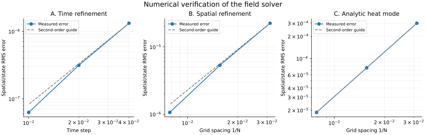
Field Responses and Mechanism Ablations
This section reports the primary comparison and every prespecified mechanism and retention-time variant. The outcomes describe the chosen parameter regime and preserve the distinction between an analytic existence argument and a numerical magnitude.
The maximum difference in both accessible fields is exactly zero throughout the matched window, as is the difference in
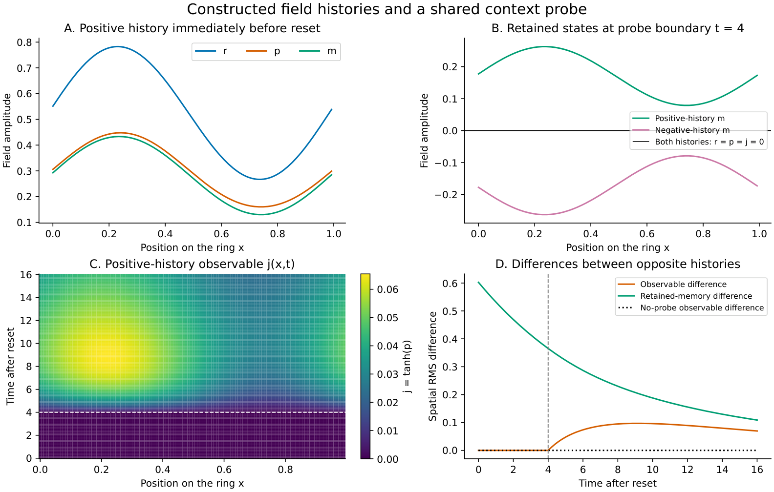
Each ablation reruns its own exposure and preparation phases. Removing interpretive feedback by setting
Changing
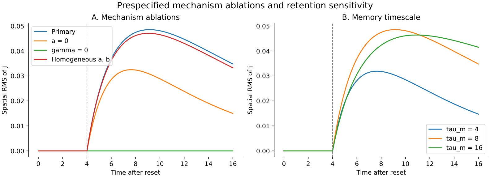
Interpretive Limits and Empirical Development
This section identifies the model’s contribution to the philosophical paper and the evidence required for further application. It examines the observation regime, the supplied interpretive architecture, and the relation to the independent live-agent study.
The model supplies a precise case in which evolving relational conditions form a disposition state, retained exposure affects later responses, and interpretive output participates in subsequent relational conditions. Observable agreement is indexed to the disclosed variables and available controls. This conditional lesson can inform Paper I’s discussion of manifest agreement and generative history. The simulation cannot determine which aspects of an actual human or artificial system have these dynamics.
The reset and context gate are decisive idealisations. A practical analogue would require evidence that an intervention can equate the accessible state while preserving a relevant latent state. Measurement leakage, incomplete reset, and direct access to memory would change the comparison. A scalar disposition with a predetermined response function captures only state formation within an interpreter design supplied by the modeller. It does not explain the emergence of categories, semantic content, language, consciousness, or a complete system of evidential standards. The interaction metric, coefficient heterogeneity, and fixed coupling architecture are also assumed. Empirical field modelling would require justified aggregation, independently observable inputs and responses, and competing models tested under interventions.
The live-agent experiment elicits language-model responses to specified prompts. Its responses may bear on sensitivity to disclosed histories and comparison criteria. No mapping from those responses to
Reproducibility and Source Access
This section identifies the executable record and the scope of source verification. The simulation is deterministic and requires Python, NumPy, and Matplotlib. From the repository root, run python experiments/field_theory/simulate.py. The local protocol was saved before execution; it was not registered externally. The output manifest records UTC timestamps, configuration, software versions, source and protocol hashes, and hashes of generated outputs. Compressed arrays retain every recorded field profile, and JSON and CSV files retain all reported conditions and verification results. PDF and PNG figures are standalone exports. All prespecified conditions were executed; the numerical checks passed without a change to model parameters or protocol.
Bibliographic details and the permitted scope of each attribution were verified online before insertion. The Amari article was checked through its publisher metadata and abstract; no full-text derivation from that article is claimed. The original Wilson–Cowan article was inspected in the university-hosted PDF. The source ledger records both access limits.
Comparison Objects and Preserved Structure
This section identifies the objects compared and defines the principal relations used in the experiments. The method combines explicit mathematical definitions with counterexamples to overly broad inference from a shared property.
A field model includes a domain, state space, evolution law, admissible initial and boundary data, controls, and observation procedures. Its numerical approximation additionally specifies spatial and temporal resolution. A comparison can concern two states within a model, two complete trajectories, two evolution laws, or two descriptions of an underlying system. Equality at one level can leave another unresolved. The distinction between behaviour, representation, and latent variables has an established place in systems theory (Willems 1991).
For a deterministic autonomous model, write
Oriented-orbit equivalence also permits a strictly increasing change of time along trajectories. Its simplest form replaces the second clock by
Observations, Interventions, and Approximation
This subsection defines a finite-horizon output comparison and explains its quantifiers. It distinguishes certified relations among models from agreement in a finite set of simulated tests.
Suppose the models have common output space
Simulation and bisimulation in formal systems theory additionally require matching transitions while preserving observations; a bisimulation supplies matching in both directions. Approximate forms relax observational equality through a defined metric (Girard and Pappas 2007). The numerical studies below do not implement a general bisimulation algorithm. Their exact claims follow from direct identities for the constructed models; their sampled metrics retain their limited domains.
An error threshold generally defines a similarity relation with different logical properties from equivalence. For example, scalar values
Variational, Boundary, and Normative Comparisons
This subsection locates energy, action, and boundary comparisons within the same account of preserved structure. Table 3 records the distinctions used throughout the comparative appendices.
An energy functional, an action functional, and an accumulated scalar value describe different objects. Equality of energies leaves mobility and dissipation unspecified. Equality of an action on one path leaves its value on other paths and its variational derivatives unresolved. Equality of full action functionals under a specified path map is a stronger statement whose consequences also depend on boundary conditions, admissible variations, and, for stochastic or quantum state sums, the measure and normalization.
Boundary equivalence compares complete boundary functionals or operators after internal variables have been integrated. It can hold while insertion observables in the interior distinguish the models. A renormalization or refinement-consistency claim must identify the coarse maps and the observables they carry. Such a claim for one finite family does not establish invariance across every complex or a continuum limit. These structural requirements are explicit in spin-foam coarse-graining work (Bahr 2014).
| Comparison | Preserved structure | Further information required |
|---|---|---|
| Coordinate conjugacy | Complete forward evolution under an invertible map and a common clock | Meaning-preserving readouts, control maps, and admissible state identification |
| Oriented orbits | Trajectory images and direction under a declared time change | Physical clock, durations, scheduled inputs, and exposure |
| Observable behaviour | Output paths or laws under specified preparations and controls | Hidden state, excluded interventions, and wider horizons |
| Approximate similarity | A declared error bound under fixed metric and quantifiers | Tolerance choice, coverage, and consequences of residual error |
| Attractor agreement | A specified asymptotic set or pattern | Transient paths, rates, basins, and finite-time consequences |
| Energy or action comparison | A specified functional, its stationary structure, or a scalar evaluated on a path | Mobility, variations, metric or noise, boundary terms, and measure |
| Boundary state sums | An identified boundary functional or operator | Interior insertions, normalization, and untested boundaries or refinements |
| Norm-relevant similarity | Legally or ethically material properties under a defended rule | Authority, evidence, exceptions, and contestability of the rule |
Comparison Structures for Field Evolution
This section distinguishes mathematical relations between field evolutions through explicit constructions on a periodic ring. Each comparison specifies the field state space, observation map, temporal convention, and admissible transformation. Exact conclusions follow from direct operator identities. The numerical examples illustrate their consequences and verify the implementation; empirical applications require an additional interpretation of the field variables and observations.
State Space and Observation Metrics
This subsection fixes the domain and distance conventions used throughout the constructions. Let the spatial domain be the ring
Fixed Spatial Coordinate Conjugacy
This subsection constructs a field equivalence under a fixed translation and examines the corresponding observation map. Define
The numerical example takes
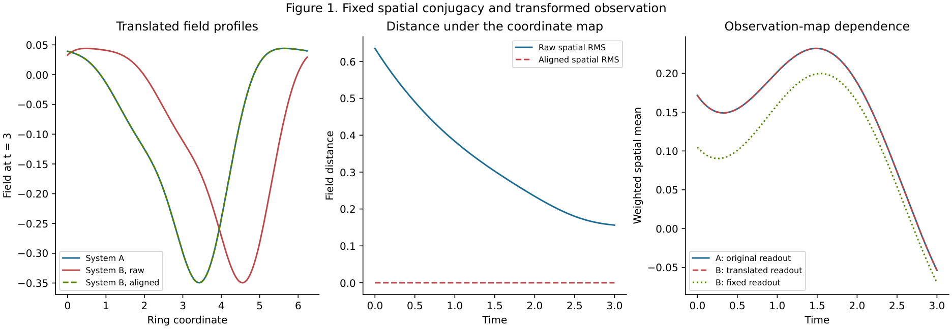
Autonomous Time Reparameterisation
This subsection compares the temporal ordering of states with their physical timing. For
Figure 5 uses
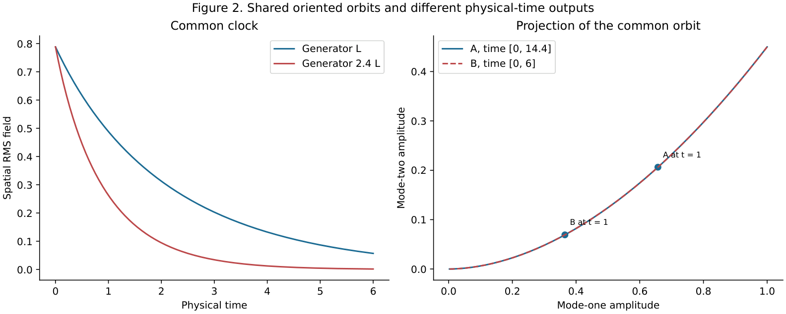
Observed Trajectories and Generator Identification
This subsection constructs complete trajectory agreement under one initial condition and separation under a declared probe. A Fourier mode
A reset to the common initial field
Under the additional assumption that the generator belongs to this known two-parameter family, rates for two distinct modes identify the parameters. For modes one and two,
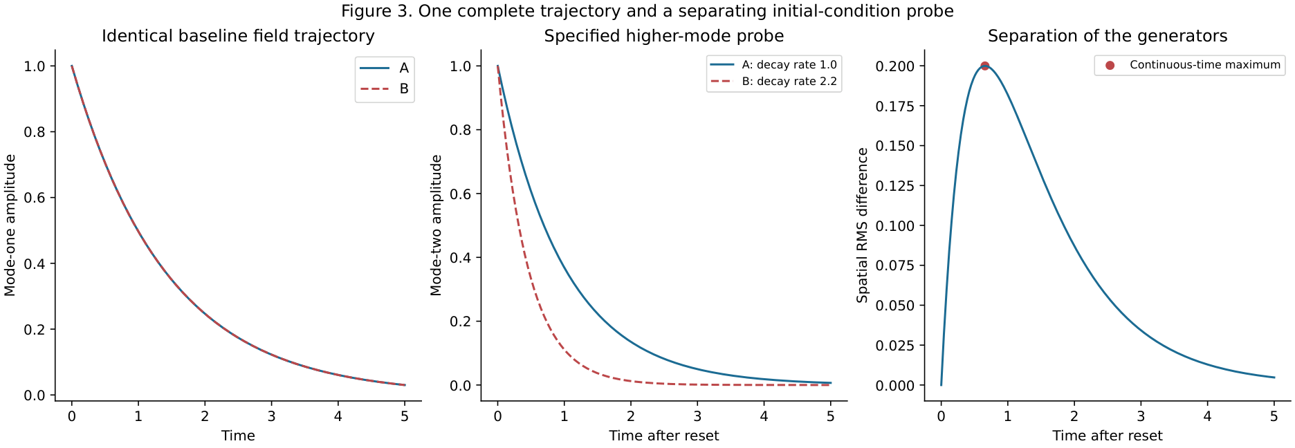
Horizon, Readout, and Admissible Translation Classes
This subsection quantifies approximate similarity under distinct comparison conventions. Consider the common initial field
The effect of an admissible fixed translation is evaluated with the time-averaged metric. Write
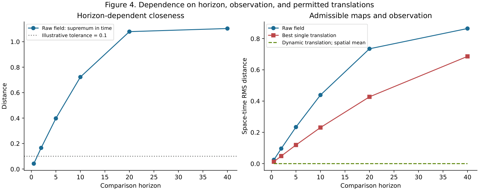
Attractors and Accumulated Observations
This subsection compares asymptotic agreement with path-sensitive quantities. Two heat-decay equations with
The exposure interpretation is illustrative. A connection to harm, opportunity, or obligation requires separately justified measurements and a normative rule. Attractor equality alone provides no such rule. The result instead identifies a mathematical distinction that a history-sensitive empirical or legal comparison may need to retain.
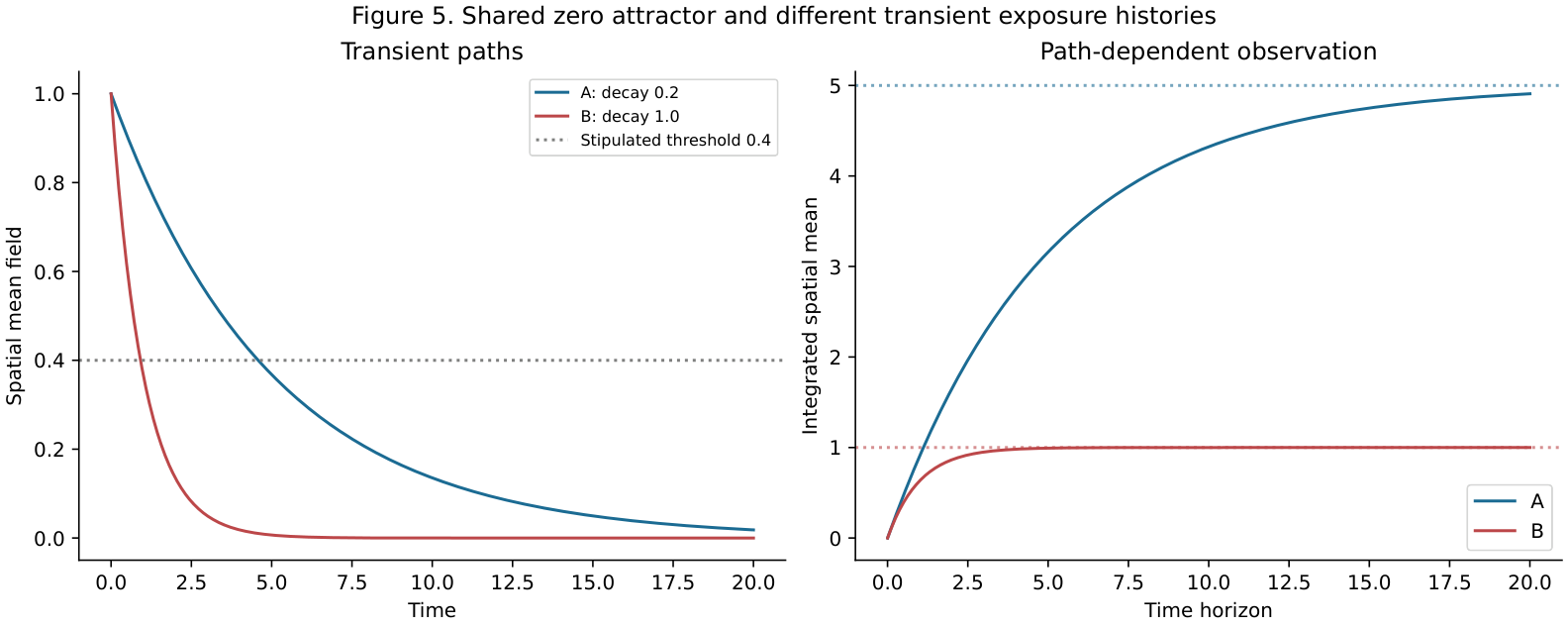
Numerical Evidence and Analytical Scope
This subsection records the evidential status and reproducibility of the computations. The heterogeneous translated system uses
Successive time-step refinement ratios are experiments/field_equivalence/.
The scalar fields isolate comparison structures alongside the project’s earlier three-field phenomenological model. They make no assertion that human and artificial systems instantiate the same equations. They establish specified identities and counterexamples, while leaving empirical field construction, admissible transformations, and norm-relevant observations to further substantive argument.
Action, Mobility, and Field Comparison
This appendix develops action-based comparisons for a specified class of dissipative fields. Its method combines a variational specification with analytically controlled numerical examples, separating stationary states, trajectories, physical clocks, stochastic temporal laws, and scalar action values. The construction supplies mathematical support for the discussion of generative relations. Application to social or interpretive fields requires independent justification of the state variables, dynamics, observables, and admissible interventions.
Variational Structures and Comparison Data
This subsection specifies the variational objects used in the comparison and their domains of interpretation. A classical stationary-action formulation selects histories by the vanishing first variation of an action under prescribed boundary variations. A gradient-flow formulation specifies an energy together with a dissipation mechanism; the latter converts energy derivatives into velocities (Tong 2004; Peletier 2014). Consequently, an energy alone leaves temporal evolution underdetermined. The numerical construction below uses positive symmetric mobility and makes no claim that the programme’s separate nonsymmetric, coupled three-field system admits this structure.
Let
For a continuously differentiable trial history on
The same expression is the small-noise rate action for the finite-dimensional diffusion
Expanding the square connects residual action to dissipation and endpoint energy, as shown in Equation 21.
Shared Energy and Temporal Structure
This subsection compares the exact field evolutions generated by the three mobilities. All runs use
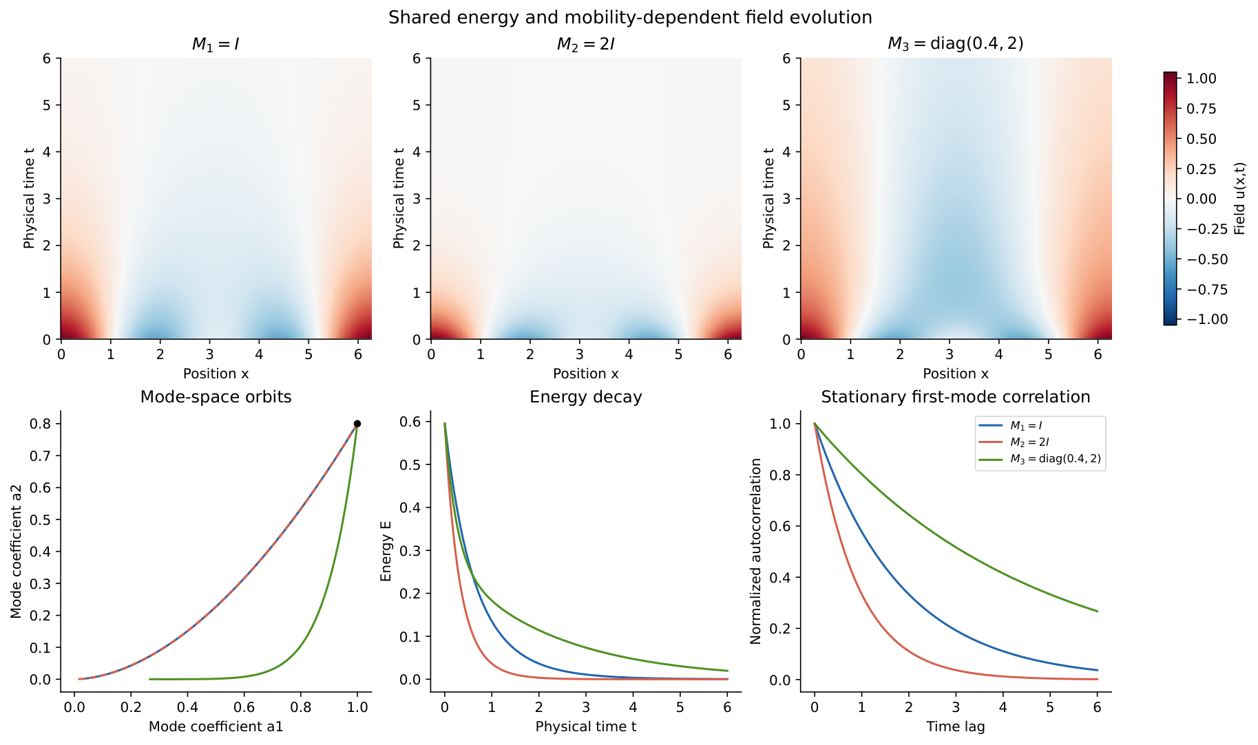
All three mobilities share the energy functional and its unique stationary field,
The unequal-mode mobility changes the initial tangent direction: the sine of its angle with the reference tangent is
An explicit alternative identification clarifies this qualification. On the selected coefficient space, the homeomorphism
The diffusion extension illustrates an additional distinction. For each mobility its stationary law is Gaussian with covariance
Scalar Action and Historical Distinction
This subsection evaluates action as a comparison statistic and constructs histories occupying the same action level set. Table 4 first evaluates each deterministic history under each candidate generator, using Equation 20 with a common field identification, initial condition, and physical interval.
| Generating mobility | Action under |
Action under |
Action under |
|---|---|---|---|
| 0 | 0.07432806 | 0.10179066 | |
| 0.07437521 | 0 | 0.21999995 | |
| 0.09745974 | 0.20430053 | 0 |
Every history has zero residual action under its own generator. Equality of these diagonal entries expresses successful evolution under three separately specified equations. It does not establish equality of those equations. The off-diagonal comparisons supply additional information about disagreement under a common state interpretation. Their asymmetry also shows that this cross-evaluation is a directed discrepancy, rather than a metric on models. A similarity analysis may use it only with an explicit reference generator, path ensemble, time interval, and normalization.
To test scalar action under one common functional, consider two trial paths on
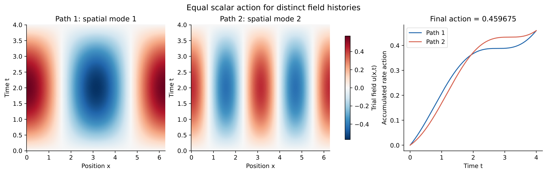
Coordinate Maps and Boundary Contributions
This subsection identifies structural information needed when action comparisons permit changes of representation. For an invertible constant linear coordinate map
Classical stationary-action equivalence involves a different comparison. Adding a total derivative to a Lagrangian shifts its action by
A direct calculation also qualifies the information supplied by a complete rate functional restricted to a boundary class. For
Verification and Scope of Interpretation
This subsection documents numerical verification and the scope of the illustrative conclusions. The protocol preceded the numerical execution. Main trajectories use exact exponentials; analytic time derivatives and integrals independently check residual-action quadrature. The maximum cross-action quadrature error is
A separately timestamped post-run audit records the subsequently observed software environment and hashes of the preserved output files. It is a retrospective artifact audit, distinct from the execution-time record embedded in the numerical results. The analytic conjugacy and boundary-class qualifications above were added during integration without rerunning or replacing those outputs.
The simulation supports carefully scoped mathematical distinctions: a shared equilibrium or energy leaves mobility open; a shared orbit leaves its physical clock open; a shared stationary marginal leaves temporal correlations open; and a shared scalar action leaves the intermediate history open. A field similarity claim should state which of these structures it preserves, which transformations it admits, which histories or interventions it tests, and which norm and tolerance it uses. The examples introduce no new empirical claim about consciousness or normative standing. Their role in the discussion papers is to discipline the meaning of relational and historical comparison. Established variational and stochastic theories supply antecedents; conceptual priority is not asserted, and objections and corrections remain welcome. The paper’s AI-use disclosure, licensing notice, and Responsible Use and Rights Reservation apply to this computational appendix.
Finite-Group State Sums and Boundary Equivalence
This section constructs an exactly enumerable field model that separates boundary equivalence from interior statistics. It first identifies the representation-theoretic structure, then derives the boundary amplitude and gluing rule, and finally compares two distinct microscopic models. The construction uses a classical positive-weight finite-group system. Its relation to spin foams is mathematical and explicitly limited.
Group Variables, Action, and Representation Labels
This subsection defines the degrees of freedom, measure, and action. It specifies the structural content that makes a dual spin-foam-type description available.
Take a strip of
For
The irreducible characters are
Boundary Functionals and Composition
This subsection derives the complete boundary functional and identifies the effect of eliminating internal variables. The chosen normalization is retained throughout the calculation.
Let
The kernel
Identical Boundaries and Distinct Interior Laws
This subsection compares two microscopic coupling assignments and the observables retained or lost by their common boundary description. It reports both the exact analytical comparison and the executed enumeration.
The assignments
An interior insertion has conditional expectation
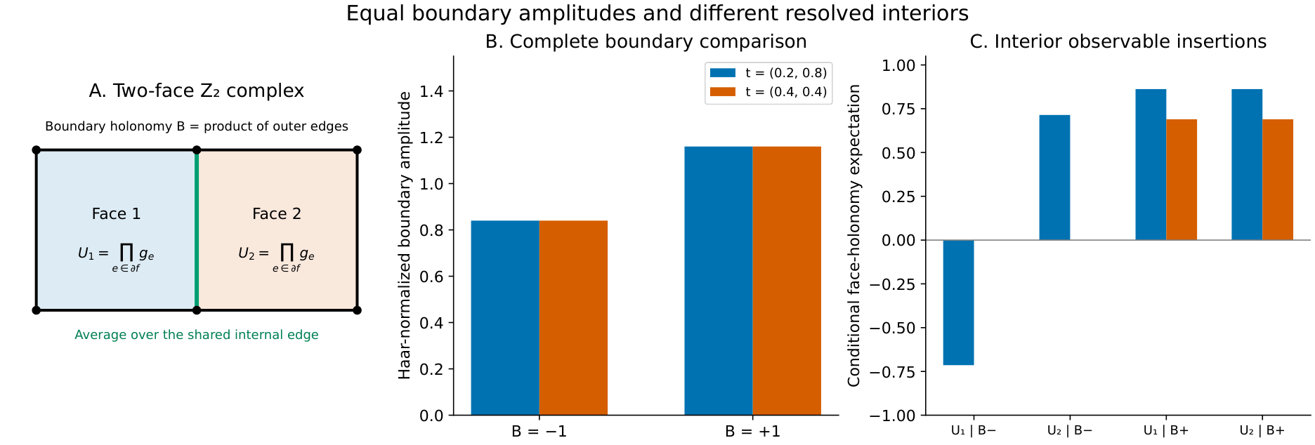
The corresponding stronger comparison can be expressed by introducing sources for interior observables. Define a source-dependent amplitude and its first insertion through Equation 26.
Figure 12 displays the continuous family
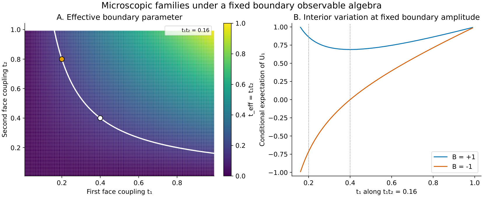
Verification and the Scope of Spin-Foam Methods
This subsection records the finite checks and the interpretation permitted by the constructed model. It distinguishes the direct mathematical transfer from claims about gravitational dynamics.
Direct edge enumeration and dual character evaluation were compared for 48 strip conditions with one through eight faces, positive, signed, and zero couplings, and both boundary signs. Their maximum absolute discrepancy was experiments/spinfoam_toy/.
This finite construction uses a two-complex, group characters, invariant constraints, a boundary kernel, and a controlled sum over internal labels. These structures support precise comparisons between representations and resolutions. In gravitational spin-foam models, boundary states and amplitude composition require additional geometric and representation-theoretic data (Perez 2013). Even semiclassical connections to an action depend on the model and boundary regime: the EPRL four-simplex asymptotics studied by Barrett and colleagues contain multiple Regge-related contributions and prefactors (Barrett et al. 2009). A universal replacement of every amplitude by a single exponential of a chosen action would therefore omit material structure.
For the discussion papers, the transferable proposal is to make boundary data, hidden histories, admissible maps, and insertion observables explicit. A social interpretation of the group variables would require its own evidence and mapping. The present positive weights define a classical statistical model; they supply no oscillatory quantum amplitudes, gravitational geometry, or explanation of consciousness. The demonstrated boundary and interior distinction remains mathematically informative within that deliberately limited scope.
Interpretation and Computational Records
This appendix records the scope and reproducibility of the shared mathematical studies.
Relational Interpretation and Issue-Relevant Equivalence
This section connects the mathematical comparisons to the companion discussion papers. It identifies the proposed analytical use and the substantive premises that the formal results leave open.
For Paper I, a reality comparison should identify which observations, relations, or interventions justify treating two entities alike. An equal recorded history need not identify its generator, whereas a coordinate difference can arise between descriptions that preserve the complete dynamics. Both distinctions matter: different appearance can accompany an equivalent description, and matching appearance can accompany different mechanisms. The appropriate conclusion depends on the declared comparison, rather than the word equivalence alone.
The action and finite-group calculations extend this argument to history-sensitive descriptions. An action can organise possible paths, and a boundary state sum can aggregate unresolved interiors. Their availability does not make every retained difference empirically accessible or relevant to a reality judgment. Conversely, equality of the selected aggregate cannot settle all questions about those interiors. The original three-field memory experiment remains a distinct example with its own state reset and context gate; the new studies examine equivalence between model descriptions more broadly.
For Paper II, an admissible comparison map must preserve the roles, time scales, options, and evidential distinctions material to the governing issue. A clock rescaling that removes a period of deprivation can destroy legal relevance while preserving an orbit. A boundary record that retains only a final agreement can erase the history through which agreement became available. The field representation should therefore make its observation map and omitted information inspectable. The legitimacy of a legal classification remains dependent on a norm and its institutional authority.
The numerical examples are constructed counterexamples and exact model identities. They are independent of the earlier 24-agent pilot and have no fitted relationship to its language outputs. They do not identify social dynamics as gravitational fields, establish a quantum mechanism of interpretation, or demonstrate consciousness. Their contribution is a disciplined set of comparison choices that can be tested and criticised before empirical or normative application.
Computational Records and Verification
This section identifies the executable record and the distinction between analytic claims and numerical checks. The field-equivalence, action, and finite-group experiments each preserve a local pre-run protocol, source code, arrays or exact enumerations, software metadata, results, and exported PNG/PDF figures. They use deterministic calculations and no external agent responses or fitted parameters.
The directories are experiments/field_equivalence/, experiments/field_action/, and experiments/spinfoam_toy/. The programme index in experiments/field_comparison/README.md links their reports and figures. Numerical refinements check discretized evolution; exact Fourier and finite-group calculations check the corresponding closed expressions. Finite tests supplement the analytic arguments and leave their stated function spaces, controls, and normalization intact. Source ledgers record the internet verification completed before citations were inserted.