A Social Spin Foam Model for Power Analysis and Governance Decision-Making
Abstract
Governance addresses social facts that are heterogeneous in kind, relational in constitution, event-laden, and observed only in part. A state vector, a network, or a single causal model represents some of these features and not the others together. This paper develops a representation in which social facts of any type are carried by the faces of a two-complex, couplings between them are carried by edges, and joint compatibility among several coupled facts is carried by vertices, so that ontological type is independent of geometric dimension and higher-order structure, including relations among relations, is expressible without special provision. Admissibility of a coupling is shown to be the support of a non-negative edge weight, which unifies the type discipline with the weighting. Weights over histories of such structures are then defined, with configuration weights and single-fact weights obtained by marginalisation, and a criterion is given for when alternative histories compose additively, namely the presence of a record that distinguishes them. Reconstruction of structure from observation is posed as a penalised inverse problem whose output is an ensemble of weighted candidates in place of one reconstructed reality, and a minimal case with five observed facts exhibits the reconstruction of unobserved structure from divergent outcomes among closely matched cases. Power is then defined as the capacity to redistribute weight over the space of possible configurations, measured by a divergence between distributions rather than by a difference of weights, and the three received faces of power are recovered as variation at three levels of the model: labels, admissibility, and the type system itself. Governance is distinguished from power as its organised, institutionalised and accountable exercise. Decision is treated as multi-objective search over admissible configurations, returning a set of non-dominated candidates and declining to reduce them to one. The contribution is a representation adequate to heterogeneous relational facts, a definition of power as an invariant of weight redistribution, and a decision procedure that separates what computation settles from what it cannot.
Keywords: social facts; two-complex; amplitude; power; governance; configuration search; relational ontology.
Notices
Licence. This work is made available under a Creative Commons Attribution-NonCommercial 4.0 International Licence, CC BY-NC 4.0.
Statement on the use of language models. Drafting, literature search and argumentative criticism for this paper were conducted in dialogue with large language models, specifically Claude (Anthropic) and ChatGPT (OpenAI). The claims, the structure, the selection of material and the position taken are the author’s. References cited have been checked; any that remain unverified are marked in the text.
Status of the proposal. This paper sets out a formal and computational research program. Estimation of the local weights it defines from social observation has no mature technology at present, and no claim is made that the procedures described here can be executed today on an actual society. What is claimed is that the steps run from observation of social facts, through reconstruction of relational configurations, to weight inference, power analysis and configuration search, and that these form one line of computational work.
Suggested citation. Huang, W. A Social Spin Foam Model for Power Analysis and Governance Decision-Making. Working draft.
Discussion Paper Note
This paper is a preliminary discussion paper intended to share an evolving idea and invite further dialogue, criticism, revision, and independent development.
The author does not claim exclusive epistemic ownership over the viewpoints, concepts, or lines of reasoning presented here, nor does the author claim priority as their first originator. Similar or related ideas may have appeared previously in other intellectual, cultural, or disciplinary traditions. Any legal rights retained in this work are intended to support attribution, responsible use, and protection against exploitative or harmful appropriation, and not to restrict independent inquiry, criticism, revision, or further development.
The arguments in this paper should therefore be understood as provisional and historically situated rather than definitive. Readers are encouraged to question, revise, extend, reinterpret, or independently develop the ideas presented here. Where appropriate, acknowledgment of this paper as one point of encounter in the development of related ideas is appreciated, but such acknowledgment should not be understood as granting the author epistemic ownership over the ideas themselves.
Responsible Use and Rights Reservation
The author encourages good-faith discussion, criticism, independent development, and responsible use of the knowledge presented in this work. The author does not claim exclusive epistemic ownership over the ideas or viewpoints discussed herein, nor claim priority as their first originator.
However, the author expressly reserves all rights and remedies available under applicable law with respect to uses of this work or related materials that involve unlawful conduct, harmful or abusive exploitation, improper commercial appropriation, infringement of applicable intellectual property or other legal rights, or conduct contrary to applicable national, regional, or international law.
This reservation is intended to preserve the ability to respond to misuse and harmful appropriation. It should not be interpreted as restricting legitimate academic inquiry, criticism, independent reasoning, or the further development of related ideas.
1. Introduction
A scholarship committee receives two applications with closely matching records and awards one of them. A regulator observes that a measured quantity has left its accustomed range. A ministry funds a programme and finds that enrolment rises while household debt rises with it. In each case the material available to whoever must decide consists of social facts of several kinds at once: entities, relations among them, attributes carried by those relations, events, states of affairs, and processes extended in time. The facts are observed in part, they stand in relations to one another that are themselves observable and describable, and the arrangement that produced them is not given directly by any observation of it.
Representations in use handle portions of this. A state vector represents attributes and supports dynamics while flattening relational structure. A network represents relations while treating nodes as primitive and typing all edges alike. A causal model represents dependence among variables while requiring the variables to be fixed in advance and treating relations among relations as a nuisance rather than as an object. Each of these is adequate to what it was built for, and none carries at once the heterogeneity of fact types, higher-order structure such as a relation between two relations, latent structure not present in the record, several possible successors to a present arrangement, and power understood as influence exerted through relations rather than as a quantity held by an entity.
This paper develops a representation that carries these together, and draws from it a definition of power and a procedure for governance decision. The representation is a two-complex whose faces carry social facts of any type, whose edges carry couplings between facts, and whose vertices carry the joint compatibility of several couplings at a place. Weights are then assigned to structures of this kind and to the transitions between them.
One terminological decision is made at the outset, since the word that names the framework carries two senses which the paper keeps apart. In one sense an amplitude is a magnitude of deviation: a measured quantity stands so far from an empirically established baseline, and this is a function of what is observed. In the other sense an amplitude is a weight attached to a possible history, expressing how strongly a given way of arriving at the present is supported. These belong to different levels. A deviation is computed on the BOUNDARY, meaning the observed present set against a record of the past; a history weight is defined over the INTERIOR, meaning the unobserved structure that connects one boundary to another. The distinction organises the paper’s epistemology: observation supports statements about boundary deviation directly, and statements about which history produced that deviation are statements about weights over an interior that observation constrains without determining. Sections 10 and 11 treat the two levels in turn.
The paper’s four contributions are these. Section 9 establishes that the type discipline of the representation and its coupling weights are one structure rather than two, since an inadmissible coupling is exactly a coupling of weight zero, and that ontological type may be assigned independently of geometric dimension without loss of formal control. Section 11 poses reconstruction as a penalised inverse problem whose output is an ensemble of weighted candidate structures, and Section 12 exhibits it on a minimal case where the divergence of outcomes between closely matched cases forces the reconstruction of unobserved structure. Section 13 defines power as the capacity to redistribute weight over possible configurations, measured by a divergence between normalised distributions rather than by a difference of weights, and shows that variation at the three levels of the model reproduces the three faces of power recognised in political theory. Section 14 treats governance decision as multi-objective search over admissible configurations, returning a set of non-dominated candidates, with Section 16 separating the determination such a search makes from the decision it leaves open.
2. Scope, and the discipline on borrowed apparatus
2.1 Scope
Six restrictions bound the claims of this paper.
The paper makes no physical claim. No constant, scale, dynamics or mechanism of any physical theory is applied to a society, and every borrowed term carries the social definition given here and nothing beyond it. In particular the framework does not assert that social processes obey quantum mechanics, and Section 10 declines the feature of quantum theory on which such an assertion would rest.
The paper does not claim that its procedures are executable at present. Estimating local weights from social observation has no mature methodology, and Section 17 records this among the limits rather than deferring it to future work in passing.
The paper supplies no criterion of justice and no ranking of social arrangements. Section 16 shows that the search procedure it proposes returns a set rather than a choice, and that the choice within that set requires a criterion the paper does not provide.
The type system, the repertoire of coupling kinds, and the objectives used in any search are supplied by an analyst. The paper treats their supply as an exercise of the same power it analyses, and Section 16 states this where the objectives are introduced.
No empirical result about any actual society is derived. The case of Section 12 is constructed to exhibit a procedure and describes no existing arrangement.
The paper concerns representation, reconstruction, power analysis and decision search. Normative theory, legitimacy and justice are named where the formalism reaches its boundary and are left to separate work.
2.2 The discipline on borrowed apparatus
Four rules govern the use of vocabulary drawn from lattice field theory and from the spin foam literature, and compliance with them is checkable line by line.
Each borrowed term receives a social definition before use, and the definition fixes its content entirely. Where a concept of the source theory has no counterpart here, the absence is recorded in the correspondence table of Section 9 in place of being passed over. Where the source theory is unsettled, the paper declines to lean on it. The construction is required to pass an admission test rather than a test of resemblance, so that objects said to compose do compose, conditions said to constrain are checkable, and any feature of the source theory doing no work here is excluded explicitly at the point where it would otherwise be assumed.
3. Prior formulations
Six bodies of work own parts of what follows. Each is conceded before anything is claimed, and the residue is stated at the end of the section.
Weighted models of network configurations. Exponential random graph models assign probabilities to labelled networks through statistics of their configurations, and Markov random fields on graphs supply the general form; Frank and Strauss(Frank, Ove, and David Strauss, “Markov , n.d.) and Wasserman and Pattison(Wasserman, Stanley, and Philippa Pattiso, n.d.) are the sources, and Snijders(Snijders, Tom A. B., “The Statistical E, n.d.) supplies actor-oriented models of network change. Sociology has therefore possessed weighted-configuration models of relational structure for decades, and no claim of novelty attaches to the idea of placing weights on relational structures.
Structure learning and latent structure. The reconstruction objective of Section 11 is a penalised structure-learning score. Minimum description length(Rissanen, Jorma, “Modeling by shortest , n.d.) supplies the principle for its complexity term, score-based search over graphical models supplies the procedure, and the recovery of unobserved common causes is the subject of an established literature(Spirtes, Peter, Clark Glymour, and Richa, n.d.). Averaging over structures compatible with data is Bayesian model averaging(Hoeting, Jennifer A., David Madigan, Adr, n.d.). The ensemble output of Section 11 is of that form.
Typed and higher-order structure. Atkin(Atkin, Ronald H., mph Mathematical Struc, n.d.) modelled social structure with simplicial complexes, and the higher-order network literature has developed the theme with hypergraphs and simplicial complexes(Battiston, Federico, Giulia Cencetti, Ia, n.d.). Multilayer and multiplex networks(Kivel a, Mikko, Alex Arenas, Marc Barthe, n.d.) carry edge types, so the coupling labels of Section 9 have a direct ancestor there. Typed attributed graphs and knowledge representation formalisms own the type discipline itself.
Relational and processual sociology. The treatment of an entity as a persistent pattern in relations rather than as a primitive is the position of relational sociology, stated programmatically by Emirbayer(Emirbayer, Mustafa, “Manifesto for a Re, n.d.) and developed processually by Abbott(Abbott, Andrew, mph Processual Sociology, n.d.). Section 8 adopts it and adds only a criterion of persistence.
Non-classical composition in the human sciences. Models with non-commuting operations and interference terms have been applied to judgement and decision, where they are justified by order effects and by violations of classical probability rather than by analogy with physics; Busemeyer and Bruza(Busemeyer, Jerome R., and Peter D. Bruza, n.d.) is the standard reference. Section 10 takes a position on this literature and declines the feature it is usually invoked for.
Power and directed influence. Power as the capacity to make others act otherwise is Dahl(Dahl, Robert A., “The Concept of Power,, n.d.); agenda control and non-decision are Bachrach and Baratz(Bachrach, Peter, and Morton S. Baratz, ‘, n.d.); the shaping of what can be contested is Lukes(Lukes, Steven, mph Power: A Radical View, n.d.); the distinction between a capacity and its exercise is Morriss(Morriss, Peter, mph Power: A Philosophic, n.d.). On the formal side, controllability of networked systems(Liu, Yang-Yu, Jean-Jacques Slotine, and , 7346) identifies nodes whose variation moves the reachable set, and transfer entropy(Schreiber, Thomas, “Measuring Informati, n.d.) measures directed influence between processes. Section 13 stands in a definite relation to each.
Each of the six families weights, learns, or analyses a STRUCTURE. None of them carries the three features jointly required here: a distinction between an observed boundary and an unobserved interior; joint compatibility among several couplings treated as an object in its own right rather than as a derived property; and weights defined over HISTORIES of typed structure in place of weights over structures at a moment. The claim of this paper is confined to what follows from those three.
4. Preliminaries
This section defines the apparatus used below, with a worked instance for each: two-complexes, labellings and admissible couplings, weights and their marginals, divergences between distributions, and dominance in several objectives. Each object is used only in the form defined here.
4.1 Two-complexes
A two-complex $\Cx=(V,E,F)$ consists of a finite set $V$ of vertices, a finite set $E$ of edges, and a finite set $F$ of faces, together with two incidence relations: each edge is incident to a set of vertices, and each face is incident to a set of edges. Write $E(f)$ for the edges incident to a face $f$, $F(e)$ for the faces incident to an edge $e$, and $E(v)$ for the edges incident to a vertex $v$. The dimension of a cell is $0$ for a vertex, $1$ for an edge and $2$ for a face, and no cell of dimension greater than two is used.
As an instance, take three faces $f_1,f_2,f_3$, two edges $e_{12}$ and $e_{23}$ with $F(e_{12})={f_1,f_2}$ and $F(e_{23})={f_2,f_3}$, and one vertex $v$ with $E(v)={e_{12},e_{23}}$. Two couplings meet at a single place, and the vertex is that place.
4.2 Labellings and admissibility
Let $\Tt$, $\Rr$ and $\Kk$ be finite or measurable sets. A labelling of a two-complex consists of maps assigning to each face an element of $\Tt$ and an element of $\Rr$, and to each edge an element of $\Kk$. An admissibility function is a map $C$ from tuples of labels to $\Rpos$; a labelled configuration is admissible where the value of $C$ at each edge and vertex is strictly positive, and inadmissible where any of them vanishes. Nothing in this definition requires $C$ to take only the values $0$ and $1$; Section 9 uses the intermediate values.
4.3 Weights, marginals, and normalisation
Let $\Omega$ be a countable set. A weight is a map $w:\Omega\to\Rpos$ with $\sum_{\omega}w(\omega)<\infty$. Its normalisation is the probability distribution
$$\hat w(\omega);=;\frac{w(\omega)}{\sum_{\omega’} w(\omega’)},$$
which is unchanged when $w$ is multiplied by a positive constant, so that a weight determines a distribution while a distribution determines a weight only up to scale. Given a map $\pi:\Omega\to\Omega’$, the marginal of $w$ along $\pi$ is
$$(\pi_\ast w)(\omega’);=;\sum_{\omega\in\pi^{-1}(\omega’)} w(\omega),$$
which sums the weight of everything that $\pi$ identifies. Equation 2 is used in Section 10 to obtain weights on configurations from weights on histories.
4.4 Divergence between distributions
A divergence $D$ assigns to an ordered pair of distributions on $\Omega$ a value $D(p,|,q)\geq 0$, vanishing exactly when $p=q$. The instance used below is the Kullback-Leibler divergence
$$D_{\mathrm{KL}}(p,|,q);=;\sum_{\omega} p(\omega),\ln\frac{p(\omega)}{q(\omega)},$$
defined when $p$ is absolutely continuous with respect to $q$. Divergences are invariant under a common rescaling of the underlying weights, by Equation 1, which is the property that Section 13 requires of a measure of power.
4.5 Dominance and non-dominated sets
Let $\mathbf J=(J_1,\dots,J_m)$ map a set $\mathcal G$ of candidates to $\mathbb{R}^m$, with each component to be minimised. A candidate $g$ dominates $g’$ when $J_k(g)\leq J_k(g’)$ for every $k$ and the inequality is strict for at least one $k$. The non-dominated set is
$$\mathcal P;=;{,g\in\mathcal G:\ \text{no } g’\in\mathcal G \text{ dominates } g,},$$
and Equation 4 is in general a set rather than a single element. Selecting one element of $\mathcal P$ requires information beyond $\mathbf J$, a point on which Section 16 turns.
5. The ontology of social facts
Social research distinguishes several kinds of social fact. A common list contains entities, relations, attributes, events, states and processes, and the list is used here without any claim that it is exhaustive or that its members are mutually exclusive. Write
$$\Tt={\textsc{Entity},\ \textsc{Relation},\ \textsc{Attribute},\ \textsc{Event},\ \textsc{State},\ \textsc{Process}}$$
for the set of types, with the understanding that Equation 5 is supplied by an analyst and may be replaced by another list without altering anything that follows.
Two of the six require no primitive status, and removing them clarifies the rest.
Let $\sim$ be an equivalence relation on labelled subcomplexes expressing that two subcomplexes support the same couplings and the same further compositions. An entity is an equivalence class under $\sim$ that persists across a range of the structure, in the sense that representatives of the class occur at successive stages of a history in the sense of Section 10.
The equivalence in Definition ? is deliberately behavioural: two arrangements are the same entity when nothing that can be coupled to them distinguishes them. A university is accordingly not a primitive point but a persistent class of arrangements comprising legal relations, financial relations, teaching relations, spatial arrangements, admission events, conferral events and the production of knowledge. The received order, in which an entity has attributes and then forms relations, is reversed: events, relations and their persistence come first, and entities are what remains stable under them.
A process is a subcomplex together with an ordering of its vertices induced by couplings of temporal or causal kind in the sense of Section 9.
Definition ? removes the need for a separate ontological atom: a policy-making process is a family of coupled facts with an order on the places where they meet, and nothing further.
The principal methodological commitment of the paper concerns the relation between the two lists just introduced and the geometry of Section 7.1.
The type of a social fact is assigned by a labelling and is not determined by the dimension of the cell that carries it. Formally, the typing map $\tau$ of Section 9 is unconstrained as a function into $\Tt$, and every restriction on which facts may occur together is imposed on COUPLINGS.
Assumption ? is a substantive choice, and the alternative is worth stating in order to see what the choice buys. One might fix the geometry to the ontology directly, taking vertices to be events, edges to be relations and faces to be some further category. That arrangement is simple, and it forbids exactly the structures that social description requires. An event may contain events; an entity may contain entities of the same kind, as an organisation contains organisations; and a relation may hold between two relations, as when an alliance between two parties bears on a supply relation between two firms. Writing the last of these as
$$R(R_1,R_2)$$
makes the difficulty visible: if relations are confined to edges, then Equation 6 has no place to live, since its arguments are already edges and it is itself a relation. Under Assumption ? the three facts in Equation 6 are three faces and the couplings between them are edges, and the recursion costs nothing.
The price of the assumption is that geometry no longer carries ontological information, so a reader may ask what the geometry is doing. Section 9 answers that question after the couplings have been defined.
6. The representation
A social configuration is the tuple of Equation 7,
$$\Sf=(\Cx,\tau,j,\kappa),$$
in which $\Cx=(V,E,F)$ is a two-complex in the sense of Section 7.1; $\tau:F\to\Tt$ assigns to each face the type of the social fact it carries; $j:F\to\Rr$ assigns to each face a label recording the observable or structural magnitudes of that fact; and $\kappa:E\to\Kk$ assigns to each edge the kind of coupling it expresses.
Three readings fix the content of Definition ?. A face carries a social fact of any type, so an employment relation, an award decision, a rate of unemployment and a state of emergency are all faces, differing in the value of $\tau$ and in the space in which $j$ takes its value. An edge carries a coupling, meaning a way in which two facts combine, constrain, depend on or realise one another; candidate kinds include causal, constitutive, normative, ownership, temporal, epistemic and institutional couplings, and the repertoire $\Kk$, like the type list of Equation 5, is supplied by an analyst. A vertex carries no social fact at all: it is a place at which several couplings meet, and what it records is that the facts they join are jointly instantiated there. Figure 1 shows the three kinds of cell together on a fragment of the case of Section 12.
A relation in the sociological sense, such as one party employing another, is a FACE with $\tau(f)=\textsc{Relation}$; it is observable, it carries attributes through $j$, and other facts may bear upon it. A coupling in the modelling sense is an EDGE. Keeping the two apart is what allows Equation 6 to be written: two faces of relation type joined by an edge whose kind expresses dependence between them.
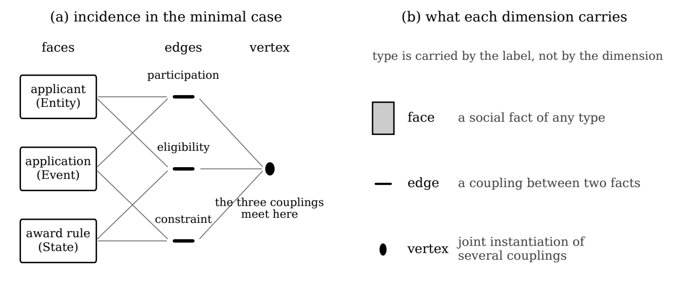
Figure 1. The three kinds of cell and what each carries. Panel (a) shows the incidence structure of a fragment of the case treated in Section 12: three social facts sit on faces, three couplings between them sit on edges, and the place where those couplings meet is a vertex. Panel (b) states the reading of each dimension. By Assumption ? the type of a fact is carried by its label and not by the dimension of the cell holding it, so an event, an entity and a state of affairs all occupy faces and differ in the value of $\tau$.
6.1 Admissibility and the weight of a coupling
Not every combination of facts may be coupled in every way. An ownership coupling between a legal status and a rate of change is ill-formed; a constitutive coupling between an event and the entity it partly constitutes is well-formed. The discipline is carried by a single function.
For an edge $e$ with incident faces $f_1,\dots,f_r$, the coupling weight is
$$C\big(\tau(f_1),\dots,\tau(f_r);,j(f_1),\dots,j(f_r);,\kappa(e)\big);\in;\Rpos ,$$
a non-negative number depending on the types of the coupled facts, on their labels, and on the kind of coupling. A coupling is admissible when the value of Equation 8 is strictly positive.
Let $C$ be as in Definition ? and let $\mathrm{Adm}$ denote the set of label tuples at which the coupling is admissible. Then
$$\mathrm{Adm};=;\operatorname{supp} C;=;{,x: C(x)>0,},$$
so a type discipline stated by a Boolean admissibility rule and a weighting stated by a non-negative function are one structure and not two: the Boolean rule is recovered as the indicator of Equation 9, and the weighting refines it by grading the admissible cases.
Immediate from Definition ?, since admissibility was defined as strict positivity. For the recovery claim, let $C_0$ be a Boolean admissibility rule; then $C=C_0$ regarded as a function into ${0,1}\subset\Rpos$ satisfies Equation 9 with $\operatorname{supp}C=C_0^{-1}(1)$. Conversely any $C$ into $\Rpos$ induces the Boolean rule $\mathbf 1[C>0]$, and the two agree on which configurations are admissible while $C$ additionally orders the admissible ones.
Proposition ? has a use beyond economy of apparatus. Social couplings are seldom permitted or forbidden outright; more often one coupling is easy to form and another is available at cost or under conditions. A Boolean rule represents the extremes and discards the intermediate cases, whereas Equation 8 represents the intermediate cases as intermediate values, and the extremes remain available as the values zero and one.
In the lattice constructions from which the vocabulary is drawn, faces carry representations of a group and edges carry intertwiners, meaning maps between tensor products of the representations meeting at that edge, which exist only for certain combinations. The role played there by the existence of an intertwiner is played here by the positivity of Equation 8. The paper takes from that construction the DISCIPLINE, namely that compatibility is enforced at the coupling in place of being written into the type system, and takes nothing else; no group, no representation theory and no invariance requirement is assumed here.
6.2 Why a two-complex
Assumption ? removed ontological content from the geometry, and the question of what the geometry contributes may now be answered.
A representation which distinguishes (i) social facts, (ii) couplings between facts, and (iii) the joint compatibility of several couplings at one place, requires cells of three dimensions, and a two-complex is the smallest structure providing them.
A structure with cells of one dimension only, meaning a set of facts with no relations, represents (i) alone. A structure with cells of two dimensions, meaning a labelled graph or hypergraph on facts, represents (i) and (ii): facts are its nodes and couplings its edges or hyperedges. It does not separately represent (iii), since a hyperedge joining several facts asserts one joint coupling among them and cannot express that two distinct couplings are jointly instantiated while remaining distinct couplings. Distinguishing the two requires an object incident to couplings rather than to facts, hence a cell of one dimension above the couplings. Taking facts as faces, couplings as edges and joint compatibility loci as vertices assigns exactly three dimensions, and no cell of dimension greater than two is needed for (i) to (iii).
Proposition ? states the price of collapsing the structure. A hypergraph model of the same material identifies the coupling of $f_1$ with $f_2$ and the coupling of $f_2$ with $f_3$ into a single hyperedge on ${f_1,f_2,f_3}$ whenever the three occur together, and the information that two separate couplings met is lost. In the case of Section 12 that information is the difference between a rule constraining an application and a committee attending to the same application.
For a vertex $v$ with incident edges $e_1,\dots,e_s$, the vertex weight $A_v$ is a non-negative function of the labels of the faces and edges meeting at $v$, expressing how strongly those couplings are jointly instantiated at one place. A vertex is admissible when $A_v>0$.
The weight of a social configuration $\Sf$ is
$$W(\Sf);=;\prod_{f\in F}A_f\big(\tau(f),j(f)\big)\ \prod_{e\in E}C_e\ \prod_{v\in V}A_v ,$$
with $C_e$ the coupling weight of Equation 8 and $A_f$ a non-negative face weight. A configuration is admissible when every factor in Equation 10 is strictly positive, and $W(\Sf)=0$ exactly when some coupling or some joint instantiation is inadmissible.
Equation 10 is local in the sense that every factor depends on the labels of one cell and its immediate neighbours, so a configuration’s weight is determined by conditions checkable cell by cell. The origin of the three families of local weights is addressed in Section 10, where the paper states plainly what supplies them.
Table 1 records the correspondence with the source vocabulary, including the concepts excluded from it.
| @p6.0cmp8.2cm@
| Lattice and spin foam vocabulary | Social configuration |
|---|---|
| two-complex | the structure carrying facts, couplings and their meetings (Def. ?) |
| face | a social fact of any type (Def. ?, Ass. ?) |
| face label, representation | observable or structural magnitudes of that fact |
| edge, intertwiner | a coupling between facts, weighted (Def. ?, Rem. ?) |
| admissibility of an intertwiner | positivity of the coupling weight (Prop. ?) |
| vertex, vertex amplitude | joint instantiation of several couplings (Def. ?) |
| local amplitude product | weight of a configuration (Eq. 10) |
| boundary of a foam | the observed part of a structure (§11) |
| sum over foams with fixed boundary | ensemble of reconstructions (§11) |
| group, representation theory, invariance | no counterpart taken |
| action principle and its variation | no counterpart taken |
| complex amplitudes and interference | taken only conditionally (§10) |
| quantisation, measurement postulate | no counterpart taken |
| continuum limit, spacetime geometry | no counterpart taken |
Table. The correspondence. Rows above the lower rule are definitional within this paper; rows below it name the concepts of the source theory that this paper excludes or takes only under a stated condition.
Two rows of Table 1 require comment. The row for intertwiners records a discipline and not a theorem, as Remark ? states: the group theory that makes intertwiner spaces computable in the physical case has no counterpart here, and Equation 8 is supplied rather than derived. The row for complex amplitudes is marked conditional because Section 10 gives a criterion under which the conditional is discharged, and reports that the criterion has not been met by any case examined here.
7. Histories, weights, and what supplies them
Section 9 attached a weight to a configuration standing alone. Governance concerns change, so the object of principal interest is a weight attached to a way of getting from one configuration to another.
A history $h$ with boundary $(\Sf_{\mathrm{in}},\Sf_{\mathrm{out}})$ is a two-complex with labels whose cells include those of $\Sf_{\mathrm{in}}$ and $\Sf_{\mathrm{out}}$ as disjoint subcomplexes, called its initial and final boundary, and whose remaining cells are its interior. The weight of a history is the product of local weights over all its cells, as in Equation 10, and is written $W(h)$.
The transition weight between two configurations is
$$\Am(\Sf_{\mathrm{in}}\to\Sf_{\mathrm{out}});=;\sum_{h}W(h),$$
the sum running over histories with the stated boundary. The configuration weight and the weight of a single fact are obtained from Equation 11 by marginalisation in the sense of Equation 2: summing over final boundaries gives a weight on initial configurations, and summing over all configurations containing a given face gives a weight on that face.
The hierarchy of Definition ? places the history weight first and derives the others, which fixes the reading of the whole framework. A statement about a configuration is a statement about the totality of ways of arriving at it, and a statement about a single social fact is a statement about the totality of configurations in which it occurs.
7.1 Coherent and incoherent composition
Equation 11 sums non-negative weights. A wider convention assigns complex numbers to histories and takes the squared modulus of their sum, and the difference between the two conventions is the presence of cancellation between alternatives. The choice is not cosmetic, and the paper settles it with a criterion rather than by preference.
Let $\Am$ be given by Equation 11 with non-negative weights, and let $H’\subseteq H$ be obtained by removing one or more histories from the sum. Then
$$\Am’(\Sf_{\mathrm{in}}\to\Sf_{\mathrm{out}});=;\sum_{h\in H’}W(h);\leq;\sum_{h\in H}W(h);=;\Am(\Sf_{\mathrm{in}}\to\Sf_{\mathrm{out}}).$$
By Equation 12, closing off an available way of reaching an outcome never raises the weight of that outcome.
Each removed term is non-negative, so the sum over $H’$ differs from the sum over $H$ by the subtraction of a non-negative quantity.
Suppose an arrangement is observed in which the removal of an available generative pathway RAISES the frequency of an outcome, with the remaining pathways unchanged. Then no model of the form of Equation 11 with non-negative weights accounts for the observation, by Proposition ?, and a convention admitting cancellation between histories becomes necessary.
Corollary ? converts a question of formal taste into an empirical criterion. The argument commonly offered for cancellation in social settings is that two measures each raising an outcome may, jointly, produce less of it than either alone. That observation is insufficient, since non-additivity of joint interventions is represented by interaction terms in models with non-negative weights and is ordinary in accounts of institutional complementarity. What Proposition ? forbids is stronger and rarer: an increase produced by removing an option.
A second consideration bears on when cancellation could arise at all. Alternative histories compose as a single sum only where nothing distinguishes them; where the arrangement carries a record of which history occurred, the alternatives are separate cases and their weights are summed after any modulus is taken rather than before.
Let $\rho$ be a map from histories to records, expressing what the arrangement retains about how it arrived at its present state. Where $\rho$ separates two histories, the two contribute to different observable cases; where $\rho$ identifies them, they contribute to one. Cancellation between histories is therefore available only within a fibre of $\rho$. Institutional settings maintain registers, minutes, ledgers and files whose purpose is to separate histories, so fibres of $\rho$ are small there and the scope for cancellation correspondingly narrow; settings without such records have larger fibres. The paper takes non-negative weights as its convention on this ground, states Corollary ? as the condition under which the convention would have to be abandoned, and reports that no case examined here meets it.
7.2 The origin of the local weights
Equation 10 is a product of face, coupling and vertex weights, and the paper owes an account of where those come from. In the physical constructions from which the form is borrowed they are derived from representation theory together with a variational principle. Neither is available here: a society supplies no action to be extremised, and the labels of Section 9 carry no group.
The paper accordingly makes no claim of derivation. The local weights are of two kinds, and the distinction between them is stated so that a reader can see which parts of an application rest on evidence and which on stipulation. A weight is estimated where it is fixed by observed frequencies of the corresponding local pattern in a body of data, in the manner in which the parameters of a weighted configuration model are fitted; the prior formulations of Section 6 supply the estimation machinery for this case. A weight is stipulated where an analyst supplies it from institutional knowledge, as when a legal impossibility is recorded by a coupling weight of zero. Section 17 records the absence of a derivation as the second most severe limit of the framework.
Three features of the source construction are used: locality, meaning that a global weight is a product over cells; the enforcement of compatibility at couplings in place of the type system; and the summation over interiors with a fixed boundary. Three are not used: the group-theoretic derivation of local weights, the variational principle, and complex amplitudes with their attendant measurement postulate. Table 1 records the exclusions, and Remark ? records the condition under which the third would be revisited.
8. Reconstruction from observation
Observation of a society yields records of facts and of some relations among them. It does not yield the structure that produced them, and the passage from one to the other is the first of the two technical problems this paper addresses.
An observation is a tuple
$$d_i=(\tau_i,\ j_i,\ \Gamma_i,\ c_i),$$
recording the type of the observed fact, its observed labels, the set of other observations to which it is observed to be coupled, and a confidence $c_i\in[0,1]$ expressing the evidential support for the record. A body of observation is $D={d_1,\dots,d_n}$.
A configuration $\Sf$ is compatible with $D$ when there is an injection from the observations into the faces of $\Sf$ preserving type and coupling. The fit of $\Sf$ to $D$ is
$$L(D\mid\Sf);=;\sum_{i=1}^{n}c_i,\ell\big(d_i,\Sf\big),$$
with $\ell$ a per-observation agreement term, so that a poorly supported observation constrains the reconstruction less than a well supported one.
Given $D$ and a complexity measure $\Omega$, the reconstruction objective is
$$\Phi_\lambda(\Sf);=;L(D\mid\Sf);-;\lambda,\Omega(\Sf),\qquad \lambda>0,$$
with $\Omega$ the description length of the configuration, counting its cells and the labels they carry. The penalty in Equation 15 is what prevents unobserved structure from being added without cost.
The problem posed by Equation 15 is ill posed in the standard sense: the map from structures to observations discards information, so its inverse is not single valued, and a penalty is required to select among preimages. Two consequences follow, and the second is the more important.
Let $\Sf$ be compatible with $D$ and let $f^{\ast}$ be a face not in the image of the injection of Definition ?. Then the configuration obtained by deleting $f^{\ast}$ together with its incident cells, where the result remains admissible, is also compatible with $D$ and attains a strictly smaller $\Omega$. Hence for a range of $\lambda$ several distinct configurations attain values of $\Phi_\lambda$ within any given tolerance, and $D$ does not determine a unique reconstruction.
Compatibility is stated by an injection from observations into faces, and deleting a face outside the image leaves the injection intact, so compatibility is preserved. Description length is monotone in the number of cells, so the deletion strictly reduces $\Omega$ while leaving $L$ unchanged, by Equation 14, since $\ell$ depends on the observed faces alone. The same argument applied to distinct unobserved faces yields distinct configurations of equal fit and equal penalty, which therefore attain equal values of Equation 15.
The output of reconstruction is the weighted family
$$\mathfrak F_D;=;\big{(\Sf_k,\ \Am_k)\big}_{k=1}^{N},
\qquad
\Am_k;\propto;W(\Sf_k),\exp!\big(\Phi_\lambda(\Sf_k)\big),$$
combining the prior weight of a configuration with its fit to observation and its complexity, normalised by Equation 1.
Equation 16 states the epistemic position of the framework in one line. Observation constrains the space of structures and assigns relative support within it, and does not return one reconstructed social reality. Proposition ? shows that the alternative is unavailable rather than merely unattractive: a procedure returning a unique structure from finite observation would have to break ties that the evidence leaves untied, and the tie-breaking would be doing work that no observation supports.
9. A minimal descriptive case
The construction is now carried out on a case small enough to state completely. The case is invented, describes no existing arrangement, and names no jurisdiction; its purpose is to show what the reconstruction of Section 11 returns when observation leaves an outcome unexplained.
9.1 The observed material
A body awards a scholarship under a published rule. Five facts are observed, and Table 2 records them in the form of Equation 13.
| @llp7.4cm@
| Face | Type $\tau$ | Observed labels and couplings |
|---|---|---|
| $f_1$ applicant A | Entity | recorded attributes; coupled to $f_4$ by participation |
| $f_2$ applicant B | Entity | recorded attributes, agreeing with those of $f_1$; coupled to $f_5$ |
| $f_3$ award rule | State | published criteria; coupled to $f_4$ and $f_5$ by constraint |
| $f_4$ application of A | Event | dated; outcome refusal |
| $f_5$ application of B | Event | dated later than $f_4$; outcome award |
Table. The observed partial configuration of the minimal case. Types are drawn from Equation 5; couplings are drawn from the repertoire of Section 9.
Four further observations bear on the case and enter the fit of Equation 14 with the confidences shown: the recorded attributes of the two applicants agree on every criterion named in the rule, with confidence $0.9$; the two decisions were taken on different dates, with confidence $0.9$; the written reasons cite the rule alone, with confidence $0.6$; and the deciding panel had the same composition on both dates, with confidence $0.8$.
The observed material is inconsistent with itself under the rule as published. Two applications agreeing on every criterion named by the rule received opposite outcomes, so some fact bearing on the outcome is absent from the record. A representation confined to what was observed has nothing to say about this beyond registering the anomaly.
9.2 Candidate unobserved facts
Three candidate faces are proposed, each of a different type and each coupled differently to the observed material:
$$\begin{aligned}
h_1&=\text{a difference in supporting testimony reaching the panel},\
h_2&=\text{a standing preference of the panel over an unrecorded attribute},\
h_3&=\text{exhaustion of the budget between the two dates}.
\end{aligned}$$
Each of the three faces in Equation 17 accounts for the divergence, and each is coupled to the observed faces in its own way: $h_1$ by an epistemic coupling to the two application events, $h_2$ by a normative coupling to the panel and thence to both events, $h_3$ by a temporal coupling to the two dates.
Candidate configurations are the non-empty subsets of Equation 17 adjoined to the observed partial configuration, giving seven candidates, of which Figure 2 draws the observed material together with the three positing a single unobserved fact. Prior weights for the formation of each hidden face are stipulated in the sense of Section 10.2, at $0.60$, $0.35$ and $0.45$ respectively; per-observation agreement is scored in $[0,1]$; and the complexity penalty of Equation 15 charges two cells for each hidden face, one for the face and one for its coupling, at $\lambda=0.35$.
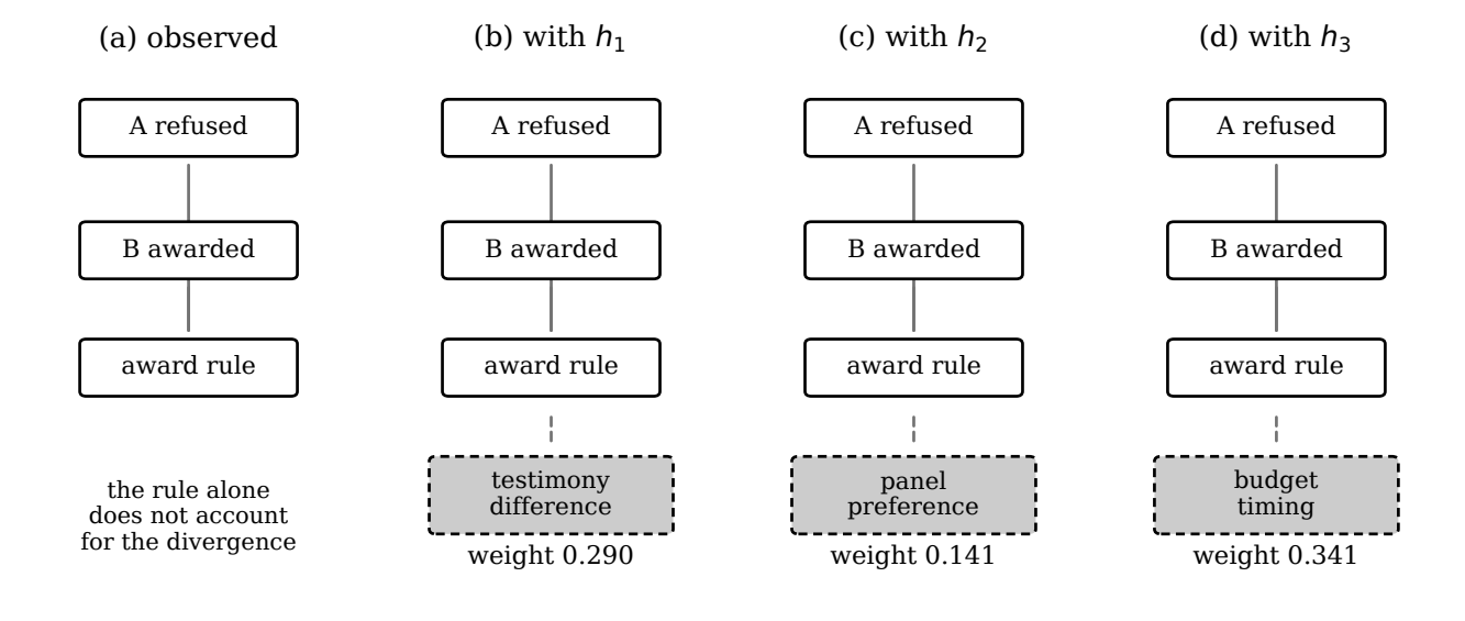
Figure 2. The observed material and three of the seven candidate reconstructions. Panel (a) contains only what was observed, and the award rule alone leaves the divergence of outcomes unaccounted for. Panels (b) to (d) each adjoin one unobserved fact from Equation 17, drawn with a broken outline, together with the coupling that carries it. The weights beneath are those computed in Table 3, and they are the weights of the candidates positing exactly one unobserved fact.
9.3 The reconstruction ensemble
Applying Equation 16 to the seven candidates yields the ensemble of Table 3.
| @lrr@
| Candidate configuration | Objective $\Phi_\lambda$ | Ensemble weight |
|---|---|---|
| observed material with $h_3$ | $2.320$ | $0.341$ |
| observed material with $h_1$ | $1.870$ | $0.290$ |
| observed material with $h_2$ | $1.690$ | $0.141$ |
| observed material with $h_1,h_3$ | $1.620$ | $0.101$ |
| observed material with $h_2,h_3$ | $1.620$ | $0.059$ |
| observed material with $h_1,h_2$ | $1.170$ | $0.050$ |
| observed material with $h_1,h_2,h_3$ | $0.920$ | $0.018$ |
Table. The reconstruction ensemble of Equation 16 for the minimal case, normalised by Equation 1. Two candidates attain equal values of the objective and differ in ensemble weight through their prior weights, which illustrates Proposition ?.
Four features of Table 3 carry the argument of the paper.
The output is a distribution and not a reconstruction. No candidate holds a majority of the weight; the leading candidate holds $0.341$ and the next $0.290$, so the evidence discriminates weakly among three explanations and the framework reports that fact in place of concealing it behind a selected structure.
Aggregation across candidates answers questions that no single candidate answers. The weight resting on configurations that contain a standing preference of the panel is $0.268$, obtained by summing the four rows in which $h_2$ appears. That quantity is the marginal of Equation 2 applied to a single face, and it is the quantity a reviewer of the decision would want, since it concerns the presence of the fact rather than the identity of the whole configuration.
The complexity penalty does the work assigned to it in Section 11. Configurations positing two hidden facts carry lower weight than either of their parts alone, and the configuration positing all three is the lightest of the seven at $0.018$, so a reconstruction is not improved by adding structure that the observations do not require.
Ties in the objective are broken by prior weight rather than by fiat. The candidates with ${h_1,h_3}$ and ${h_2,h_3}$ attain the same value $1.620$ of Equation 15 and receive different ensemble weights, $0.101$ against $0.059$, because Equation 16 multiplies the fit by the prior weight of the configuration. Where prior weights are absent the two would remain tied, which is Proposition ? in a concrete instance.
A knowledge graph of the material in Table 2 records five facts and their couplings and stops there. The reconstruction returns seven weighted structures, four of which contain a fact that appears in no record, and assigns to the presence of that fact a definite weight. The procedure is the recovery of latent relational structure, and the anomaly in the observed material is what makes the recovery possible: a case in which the rule accounted for both outcomes would leave the hidden faces unsupported and their weight would fall to the prior.
10. Power
Power is treated here as a property of a position in a structure rather than as a possession of an entity, and it is measured by what varying that position does to the distribution over possible configurations.
10.1 Two corrections to the natural definition
The natural first definition takes the difference of weights produced by varying a fact. Two features of the present setting require it to be amended.
Types, couplings and the presence or absence of a face are discrete, so a derivative with respect to them is undefined. The definition below is stated with a difference operator, and a derivative is recovered as its limiting case where a label varies in a continuous space.
Let $W$ and $W’=cW$ for $c>0$ be two weightings differing by a scale. Then for any configurations the difference $W’(\Sf)-W(\Sf)$ depends on $c$, while the normalised distributions $\hat W$ and $\hat{W’}$ of Equation 1 coincide. A measure of power defined as a difference of weights therefore reports a change where none has occurred in the relative standing of any configuration.
$W’(\Sf)-W(\Sf)=(c-1)W(\Sf)$, which is non-zero for $c\neq 1$ wherever $W(\Sf)>0$; and $\hat{W’}=\hat W$ by Equation 1, since the constant cancels between numerator and denominator.
Proposition ? fixes the form of the definition: what must be compared is the distribution before and after, and the comparison must be by a quantity insensitive to a common rescaling. Section 7.4 supplies such a quantity.
Let $\Am$ be the weight over configurations of Definition ?, let $x$ be a face, a coupling, a label or an admissibility rule, and let $\Am_x$ be the weight obtained when $x$ is varied by a specified act. The power of that act is
$$P_x;=;D\big(\hat\Am_x,\big|,\hat\Am\big),$$
the divergence of the resulting normalised distribution from the original. The directed influence of $x$ on a fact $y$ is Equation 18 computed on the marginal distributions over configurations containing $y$, written $I_{x\to y}$.
Equation 18 measures capacity and not exercise: it reports what an available act would do, whether or not it is performed. The distinction is the one drawn in the literature conceded at Section 6, and the framework takes the capacity side of it.
For two facts the normalised asymmetry is
$$\Pi_{xy};=;\frac{I_{x\to y}-I_{y\to x}}{I_{x\to y}+I_{y\to x}};\in;[-1,1],$$
which is $0$ where the two influence one another equally and approaches $\pm 1$ as one of the two directions vanishes.
Equation 19 is used in preference to the ratio of the two influences, which diverges precisely in the case of greatest interest, namely where one direction of influence is near zero.
10.2 Power in the minimal case
Definition ? is now computed on the case of Section 12. Varying a hidden fact means suppressing its formation, implemented by scaling its prior weight by a factor of $0.25$, and the resulting ensembles are compared with Table 3 through Equation 3. The influences are
$$P_{h_3}=0.1985,\qquad P_{h_1}=0.1794,\qquad P_{h_2}=0.1083,$$
so that suppressing the budget-timing fact redistributes the ensemble most and suppressing the panel preference redistributes it least. The normalised asymmetry of Equation 19 between the strongest and the weakest of the three is $+0.294$.
The ordering in Equation 20 is not the ordering of the ensemble weights in Table 3, and the divergence is instructive. A fact may hold a large share of the ensemble weight while its suppression leaves the remaining distribution largely as it was, since other candidates absorb the displaced weight in similar proportions; and a fact of modest weight may hold the distribution in place. Power in the sense of Equation 18 is a property of the redistribution and not of the share.
10.3 Four kinds of act, and three levels of the model
Acts that alter Equation 18 fall into four kinds. Amplification raises the weight of certain configurations, as funding, recognition, infrastructure and access to information do. Suppression lowers it, in the limit to zero. Redistribution lowers some and raises others while leaving the total unchanged, which is the form taken by most instruments that reallocate rather than expand. Coupling acts change which facts may be joined at all, leaving the labels untouched; the questions of who may enter an institution, who may obtain credit, who may publish, who takes part in a decision, and which records may be joined to which are all of this kind.
These four are not on a level. Three of them vary the weights of configurations that remain admissible, and one varies admissibility itself. Adding the acts that vary the type system of Equation 5, the coupling repertoire, or the observables through which facts are recorded gives a third level, shown in Figure 3, and the three levels correspond to distinctions long drawn in political theory. Table 4 states the correspondence.
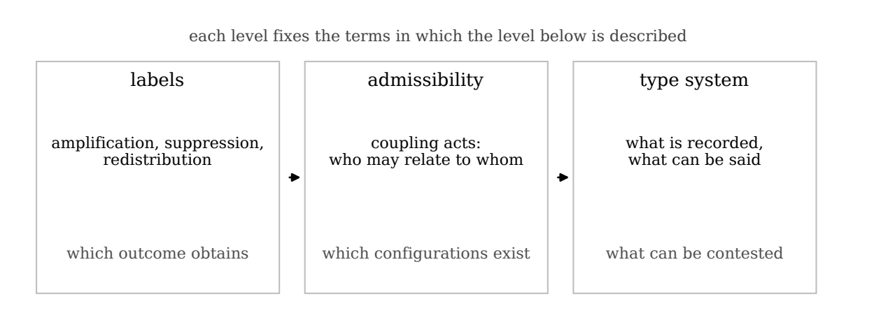
Figure 3. Three levels at which an act may vary the arrangement, with the effect of each. An act on labels settles which of the available configurations obtains; an act on admissibility settles which configurations are available; an act on the type system and the observables settles what can be recorded and therefore what can be claimed. Each level supplies the terms in which the level to its left is described, which is why the rightmost is the hardest to contest from within the arrangement.
| @p3.5cmp5.0cmp5.4cm@
| Level of the model | What is varied | Received description |
|---|---|---|
| labels | $j$ on admissible configurations; amplification, suppression, redistribution | prevailing in a decision over the resistance of others(Dahl, Robert A., “The Concept of Power,, n.d.) |
| admissibility | the coupling weight of Equation 8, hence which configurations exist | control of the agenda and the non-decision(Bachrach, Peter, and Morton S. Baratz, ‘, n.d.) |
| type system and observables | $\Tt$, $\Kk$, and the space $\Rr$ in which facts are recorded | shaping what can be described and therefore contested(Lukes, Steven, mph Power: A Radical View, n.d.) |
Table. Variation at three levels of the model, and the three faces of power to which each corresponds. The correspondence is offered as a reading of the received distinctions in the terms of this framework, not as a claim to have derived them.
The third row of Table 4 is the one the framework makes newly visible. An act at that level alters which social facts are recorded and which couplings are expressible, and a fact absent from $\Tt$ or an attribute absent from $\Rr$ cannot enter any configuration, cannot receive weight, and cannot be the subject of a claim. The choice of the type system, made in Section 8 and named there as analyst-supplied, is accordingly an act of the third kind, and the framework’s own presuppositions fall within the scope of what it analyses.
Setting the coupling weight of the panel-preference fact to zero, which is what a rule forbidding the panel to consider unrecorded attributes would do, removes four of the seven candidates of Table 3 from the admissible set, by Definition ?. The divergence of Equation 18 for that act is $0.3124$, larger than any of the three in Equation 20, and the weight resting on the testimony explanation rises from $0.290$ to $0.396$ as the displaced weight is absorbed. The act operates at the second level of Table 4 and not the first: it changes what is possible, and the change in what is weighted follows from that.
10.4 Power and governance distinguished
Governance is the organised exercise of power in the sense of Definition ?, marked by four features: it is intentional, in that a deformation is aimed at; institutionalised, in that it proceeds through an arrangement that persists beyond the act; normatively directed, in that reasons of a public kind are offered for it; and accountable, in that the arrangement answers for it to someone.
Definition ? states a criterion that does not presuppose a state. A market, a platform, a recommendation system or a settled convention may hold large power in the sense of Equation 18 while satisfying none of the four features, and the framework registers such a case as power without governance. The converse case, an arrangement satisfying all four features while holding little power, is equally representable. Section 14 concerns governance in the sense of Definition ?, and the analysis of Sections 13 to 13.2 applies to power whether or not it is governed.
11. Governance as configuration search
Governance in the sense of Definition ? acts on the amplitude landscape. This section states what an act is, what searching over acts involves, and why exhaustive search is unavailable.
An intervention is a map $u$ carrying a social configuration to another, implemented by a finite list of edits of four kinds: setting a face label, adding or removing a face, setting a coupling weight, and altering the admissibility rule for a class of couplings. The intervention is available to a party when every edit in its list corresponds to an act that party may perform.
The four kinds of edit in Definition ? are the four kinds of act distinguished in Section 13.3. Setting labels and adding or removing faces are amplification, suppression and redistribution; setting a coupling weight or altering an admissibility rule is a coupling act. The space searched by a governance procedure is accordingly the space of exercises of power available to the searching party, and the taxonomy of Table 4 classifies the search variables.
The effect of $u$ on the transition weight of Equation 11 is
$$\Delta_u\Am(\Sf_i\to\Sf_j);=;\Am\big(\Sf_i\to\Sf_j\mid u\big);-;\Am\big(\Sf_i\to\Sf_j\big),$$
so that an intervention is assessed by its deformation of a field of transition weights in place of by its effect on a single outcome quantity.
Equation 21 states the difference between this treatment and one conducted on an outcome variable. A subsidy directed at participation in education alters at once the weight of a household of modest means reaching a place of study, the weight of that place of study reaching a regional labour market, the weight of a household reaching indebtedness, and the weight of an institution reaching expansion. An assessment reporting a single figure for participation reports one component of Equation 21 and is silent on the others, which are neither side effects nor externalities in the present formulation; they are further components of the same object.
Let a configuration carry $n$ faces whose labels each range over $k$ values. The number of labellings at fixed topology is $k^{n}$. Where the topology varies, the number of admissible configurations on $n$ faces is bounded below by the number of graphs on $n$ vertices whose couplings are admissible, which grows faster than any exponential in $n$. Enumeration is therefore unavailable for cases beyond the smallest.
Each of the $n$ faces receives one of $k$ labels independently, giving $k^{n}$ labellings, and admissibility can only restrict this count within a factor determined by the coupling rules. For the second claim, the number of graphs on $n$ labelled vertices is $2^{\binom n2}$, and any fixed fraction of these remaining admissible leaves a quantity growing as $2^{cn^{2}}$ for some $c>0$, which exceeds $C^{n}$ for every $C$ and all large $n$.
The case of Section 12 carries five observed faces and three candidate hidden ones, giving seven candidate configurations, so it is enumerable and was enumerated. Proposition ? states that this is a property of its size rather than of the method.
12. Multi-objective search over admissible configurations
12.1 Encoding and admissibility
A candidate intervention is encoded as a vector $g=(g_1,\dots,g_m)$ whose entries specify the edits of Definition ?: whether a coupling is established or cut, the strength assigned to it, the label given to a face, whether a body is instituted, and what threshold a rule carries. Decoding gives $\Sf_g$, and the objectives of Section 15.2 are computed on it.
Two requirements distinguish search over configurations from search over vectors of numbers.
Mutation and recombination of $g$ may produce a decoded configuration in which some coupling weight of Equation 8 vanishes, so that $W(\Sf_g)=0$ by Definition ? and the candidate carries no information for selection. A population under unconstrained variation fills with such candidates. Variation operators are therefore required to respect the coupling rules, which is the situation addressed by grammar-guided evolutionary computation and by rewriting systems on graphs, where admissible structures are those derivable in a grammar and the operators act on derivations in place of acting on the structures directly.
Evaluating a candidate requires the weights of Definition ?, each of which is a sum over histories. A search loop therefore contains a summation over structures within every evaluation, and the cost of the procedure is the product of the two. Three reductions are available and each carries a cost of its own: sampling histories in place of summing them, which introduces sampling error into the comparison of candidates; holding the topology fixed so that only labels vary, which excludes interventions that add or remove facts; and replacing the inner sum by a fitted approximation, which makes the comparison depend on the quality of that approximation. The paper claims no scalability result and records the matter among the limits at Section 17.
12.2 Objectives, and their standing
A search is specified by a vector $\mathbf J(g)=(J_1(g),\dots,J_m(g))$ of quantities to be minimised, together with the admissibility conditions of Section 9, which act as feasibility constraints in place of terms of the objective.
The standing of the components of Definition ? requires a statement that the framework cannot supply from within. Suppose the objectives are taken to be the stability of the arrangement, its resilience under disturbance, the feasibility of the transitions it requires, and the size of the intervention. Presented as purely computational quantities, the first two carry a commitment that is not computational at all. Stability and resilience both score an arrangement by its persistence, so an arrangement in which some party is durably disadvantaged scores well through the durability, and an intervention moving toward a different arrangement is penalised as a disturbance. A search using them is not neutral between the present arrangement and its alternatives; it favours the present one, and does so silently.
Every component of $\mathbf J$ is supplied by an analyst, and the choice of components is an act at the third level of Table 4, since it fixes what the search can register. The size of an intervention is the component closest to neutrality, since it counts edits and takes no position on which arrangement is preferable. The paper’s own use of stability-like quantities in the case below is accordingly labelled where it occurs.
The output is the non-dominated set of Equation 4 restricted to admissible candidates,
$$\mathcal P;=;{,g:\ \Sf_g \text{ admissible, and no admissible } g’ \text{ dominates } g,},$$
whose members are called candidate governance configurations. No member of Equation 22 is designated by the procedure.
12.3 The search on the minimal case
Four edits are made available on the arrangement of Section 12: publishing the reasons for a decision in full, which makes the written record discriminating and raises the confidence attaching to it from $0.6$ to $0.95$; forbidding the deciding panel to act on attributes absent from the record, which is a coupling act setting the corresponding weight to zero; fixing the budget across the decision cycle, which is a coupling act of the same kind; and standardising the supporting testimony, which reduces the prior weight of a difference in testimony to three tenths of its former value. The genome is the four-vector of these edits, giving sixteen candidates, of which all sixteen are admissible, one edit combination having been excluded by the requirement that some fact remain able to account for the observed divergence.
Three objectives are computed, each to be minimised: the size of the intervention, counted as the number of edits; the weight remaining on an explanation that the written record cannot exhibit, computed as the marginal weight of configurations containing a panel preference; and the displacement of the arrangement from its present form, computed by Equation 3 against the ensemble of Table 3. The second and third are labelled as supplied in the sense of Remark ?: the second favours arrangements whose records account for their own decisions, and the third favours continuity.
| @llrrr@
| Candidate | Edits performed | Size | Opaque weight | Displacement |
|---|---|---|---|---|
| $0000$ | none | $0$ | $0.268$ | $0.0000$ |
| $1000$ | publish reasons in full | $1$ | $0.258$ | $0.0006$ |
| $0100$ | forbid unrecorded attributes | $1$ | $0.000$ | $0.3124$ |
Table. The non-dominated set of Equation 22 for the minimal case, from sixteen admissible candidates. A candidate performing all four edits attains zero opaque weight at size $4$ and displacement $1.2393$, and is dominated by the third row, which attains the same opaque weight at size $1$.
Figure 4 collects the three computed results of the paper, and Table 5 exhibits the property that motivates the multi-objective treatment. The three candidates are ordered oppositely on the second and third objectives: taking no action leaves the arrangement undisturbed and leaves the unauditable explanation carrying $0.268$ of the weight, while forbidding the panel to act on unrecorded attributes removes that weight entirely at the cost of the largest displacement in the set. Publishing the reasons occupies an intermediate position, achieving a small reduction at a displacement of $0.0006$, since a more discriminating record changes which explanation the evidence supports without changing what the arrangement permits.
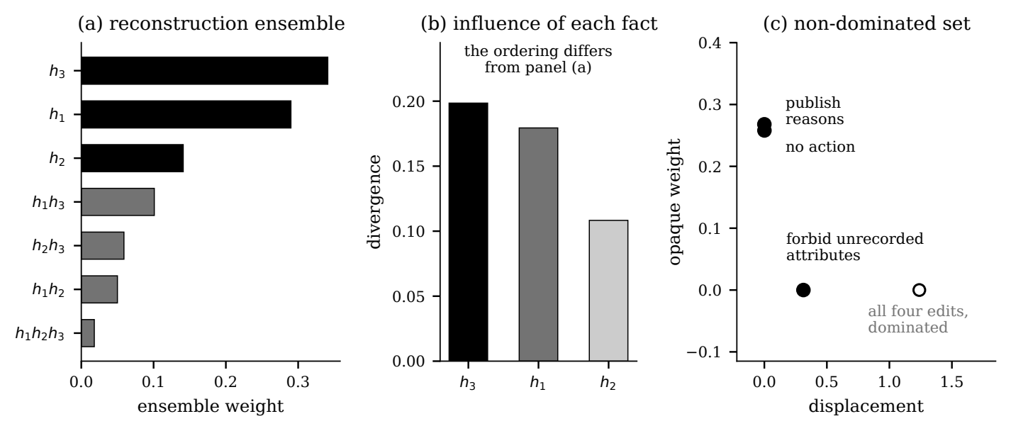
Figure 4. The three computed results. Panel (a) is the reconstruction ensemble of Table 3, with candidates positing one unobserved fact in black and those positing more in grey; the weight falls as the complexity penalty of Equation 15 takes effect. Panel (b) is the influence of each unobserved fact under Definition ?, from Equation 20; its ordering differs from panel (a), so a fact holding a large share of the weight is not thereby the fact whose suppression redistributes most. Panel (c) is the non-dominated set of Table 5 in two of its three objectives, with the candidate performing all four edits shown hollow, dominated at four times the size and four times the displacement of the candidate directly to its left.
13. The standing of a computed result
Definition ? returns a set. Selecting one member of it requires information beyond the objectives, and the following statement makes the point exactly rather than as a caution.
Let $\mathcal P$ be a non-dominated set with at least two members differing in at least two objectives. Then for any member $g\in\mathcal P$ there is a vector of non-negative weights under which $g$ minimises the weighted sum of the normalised objectives. Hence the selection of one member is determined by the weighting and not by the objectives alone.
Members of $\mathcal P$ are pairwise non-dominating, so for any two, each is strictly better on some objective. Choosing weights concentrated on an objective at which $g$ is strictly best makes the weighted sum smallest at $g$. Since the weighting is not determined by $\mathbf J$, distinct admissible weightings select distinct members.
Proposition ? is exhibited on the set of Table 5. With objectives normalised over the set, a weighting placing three times the weight on the size of the intervention selects the first row; a weighting placing three times the weight on the auditability of the record selects the third; and a weighting placing three times the weight on continuity selects the first. One set, three weightings, and two different selections, none of which is produced by the computation.
Two consequences follow for the standing of any result obtained by the method of Section 15.
A computation establishes non-domination and does not establish desirability. That a configuration cannot be improved in one respect without loss in another is a statement about the objectives supplied; it carries no implication that the objectives were the right ones, that the arrangement they favour is just, or that the party conducting the search was entitled to conduct it.
The wording of results accordingly matters. A member of Equation 22 is a candidate governance configuration or a computationally non-dominated configuration. The expression optimal social configuration is avoided throughout, since it attributes to a computation a determination that Proposition ? shows the computation does not make.
The quantities of Section 13 may enter a search in either role. Entered as an objective, a measure of concentration would rank arrangements and would carry the judgement that less concentration is better, which is a normative claim the paper does not make. Entered as a constraint, a condition such as $\Pi_{xy}\leq\theta$ rules out candidates without ranking those that remain, and the party imposing $\theta$ is visible in the specification. The constraint form is recommended on that ground, and the framework represents both.
14. Limits
Seven limits, in decreasing order of severity.
First, a baseline is conservative by construction. Any procedure that measures deviation against an established range, or displacement against a present arrangement, registers a durable arrangement as undisturbed however it distributes advantage, and registers a movement away from it as a deviation to be accounted for. Section 15.2 states this for the objectives and Remark ? labels the affected components, and the difficulty is not thereby removed. A framework of this kind is well suited to detecting departures and poorly suited to detecting settled conditions.
Second, the local weights are not derived. Section 10.2 states that they are estimated or stipulated, and the estimation route has no worked methodology for social data at present. Every numerical result in this paper rests on stipulated weights and demonstrates the procedure rather than any social fact.
Third, the type system, the coupling repertoire and the observables are supplied. Table 4 identifies their supply as an act of power, and the framework analyses such acts without exempting its own.
Fourth, the evaluation is nested and no scalability claim is made. Remark ? names three reductions and the cost each carries.
Fifth, the ensemble depends on the complexity penalty. The weights in Table 3 shift with $\lambda$ in Equation 15, and the paper offers description length as a principled choice without establishing that any particular value is correct.
Sixth, the record criterion of Remark ? is a conjecture with a motivation. It states a condition under which cancellation between histories could arise and reports that no case examined here meets the diagnostic of Corollary ?; it does not establish that no such case exists.
Seventh, no part of the framework has been applied to observed social data. The case of Section 12 is constructed, its numbers follow from stipulated weights, and its role is to show what the procedure returns rather than what any arrangement is like.
The paper’s established claims are these. A representation in which social facts of any type are carried by faces, couplings by edges, and joint compatibility by vertices supports higher-order social structure without special provision, and its type discipline is the support of its coupling weights rather than a separate apparatus. Reconstruction from observation is ill posed, so its output is a weighted ensemble and not a structure. Power is the redistribution an available act would produce, measured by a divergence between normalised distributions, and variation at the three levels of the representation corresponds to three received faces of power. Governance is the organised, institutionalised and accountable exercise of such redistribution. Search over admissible configurations returns a non-dominated set, and the selection of one member of that set is made by a weighting the computation does not supply.
References
Abbott, Andrew, Processual Sociology, University of Chicago Press, Chicago and London, 2016.
Atkin, Ronald H., Mathematical Structure in Human Affairs, Heinemann Educational, London, 1974.
Bachrach, Peter, and Morton S. Baratz, “Two Faces of Power,” American Political Science Review 56(4), December 1962, 947–952.
Battiston, Federico, Giulia Cencetti, Iacopo Iacopini, Vito Latora, Maxime Lucas, Alice Patania, Jean-Gabriel Young, and Giovanni Petri, “Networks beyond pairwise interactions: structure and dynamics,” Physics Reports 874, 2020, 1–92.
Busemeyer, Jerome R., and Peter D. Bruza, Quantum Models of Cognition and Decision, Cambridge University Press, 2012. A second edition appeared in 2024.
Dahl, Robert A., “The Concept of Power,” Behavioral Science 2(3), 1957, 201–215. doi:10.1002/bs.3830020303.
Emirbayer, Mustafa, “Manifesto for a Relational Sociology,” American Journal of Sociology 103(2), 1997, 281–317. doi:10.1086/231209.
Frank, Ove, and David Strauss, “Markov Graphs,” Journal of the American Statistical Association 81(395), 1986, 832–842.
Hoeting, Jennifer A., David Madigan, Adrian E. Raftery, and Chris T. Volinsky, “Bayesian Model Averaging: A Tutorial,” Statistical Science 14(4), 1999, 382–417. doi:10.1214/ss/1009212519. A corrected version was issued in Statistical Science 15(3), 2000, 193–195.
Kivelä, Mikko, Alex Arenas, Marc Barthelemy, James P. Gleeson, Yamir Moreno, and Mason A. Porter, “Multilayer networks,” Journal of Complex Networks 2(3), 2014, 203–271. doi:10.1093/comnet/cnu016.
Liu, Yang-Yu, Jean-Jacques Slotine, and Albert-László Barabási, “Controllability of complex networks,” Nature 473(7346), 2011, 167–173. doi:10.1038/nature10011.
Lukes, Steven, Power: A Radical View, second edition, Palgrave Macmillan, Basingstoke, 2005. First edition Macmillan, 1974.
Morriss, Peter, Power: A Philosophical Analysis, second edition, Manchester University Press, Manchester, 2002. First edition 1987.
Rissanen, Jorma, “Modeling by shortest data description,” Automatica 14(5), 1978, 465–471. doi:10.1016/0005-1098(78)90005-5.
Schreiber, Thomas, “Measuring Information Transfer,” Physical Review Letters 85(2), 2000, 461–464. doi:10.1103/PhysRevLett.85.461.
Snijders, Tom A. B., “The Statistical Evaluation of Social Network Dynamics,” Sociological Methodology 31(1), 2001, 361–395. doi:10.1111/0081-1750.00099.
Spirtes, Peter, Clark Glymour, and Richard Scheines, Causation, Prediction, and Search, second edition, MIT Press, Cambridge MA, 2000. First edition Springer, 1993.
Wasserman, Stanley, and Philippa Pattison, “Logit models and logistic regressions for social networks: I. An introduction to Markov graphs and $p^$,” Psychometrika 61(3), 1996, 401–425. thebibliography