The Geometry of Value - Loop Deficits as Invariant Measures of Structural Exploitation

Abstract

Every leg of a transfer chain can be defended as fair under some accounting, and the defences are not lies: they are re-descriptions, and re-description is cheap. Disputes about extraction therefore never terminate at a single transaction. This position paper isolates the quantities that survive re-description, by construction. Positions in a transfer network carry valuation frames; transfers carry conversion rates; a change of accounting is a gauge transformation. It is proved that the value assigned to any single leg carries no invariant content, that the entire invariant content of a transfer structure is carried by its closed loops, and that a consistent global measure of value exists exactly when every loop closes. The gauge-invariant observable is the loop deficit: the fraction of registered value lost around a closed circuit, invariant under every admissible re-description and requiring no common unit across kinds of value. The deficit is then mapped onto exploitation, and the mapping is shown to be strict in both directions: a deficit can exist without a wrong, and a wrong can exist at zero deficit. Exploitation is accordingly characterised by three joint structural conditions. A persistent deficit is absorbed at an identifiable position; that position controls the accounting schema; and return to the depleted position is blocked. For these conditions the deficit is the measuring instrument and never the verdict. The principal claim is one of localisation: since no re-description can move the deficit, every persisting dispute about extraction is a dispute about the structure of the network itself, and defences that operate by re-describing individual legs lose their purchase on it. The contribution is threefold: it gives the circulation criterion of generative justice a quantity that can be computed and compared; it explains why attribution disputes conducted at the level of transactions tend not to terminate, since their object carries no invariant content; and it converts the argument about extraction from a contest of accountings into a factual question about the structure of a network. One implication follows directly for platform economies. Computing the invariant requires the record of a whole circuit, which in such economies is ordinarily held by the intermediary alone, so disclosure of circuit-level records is the condition under which any other party can use the instrument at all.

Keywords: loop deficit; holonomy; gauge invariance; exploitation; circulation of value; generative relational economics.

Notices

Licence. This work is made available under a Creative Commons Attribution-NonCommercial 4.0 International Licence, CC BY-NC 4.0.

Statement on the use of language models. Drafting, literature search and argumentative criticism for this paper were conducted in dialogue with large language models, specifically Claude (Anthropic) and ChatGPT (OpenAI). The claims, the structure, the selection of material and the position taken are the author’s. References cited have been checked; any that remain unverified are marked in the text.

Companion papers. This paper develops the formal core of a question raised in Conditions of Future Generation in Open Knowledge Platforms: A Preliminary Discussion of a Second-Order Question in Platform Economics, which treats the economic side of an open knowledge commons and states the loop as its unit of analysis without constructing the observable. The apparatus of gauge equivalence and loop observables is developed for interpretation generally in a companion paper of the author’s on loop observables and the gauge structure of interpretation, from which the identification of redundant interpretive difference used in §7 is taken. The extension to heterogeneous value discussed in §13 is reserved for a separate treatment.

Suggested citation. Huang, W. The Geometry of Value: Loop Deficits as Invariant Measures of Structural Exploitation. Working draft.

Discussion Paper Note

This paper is a preliminary discussion paper intended to share an evolving idea and invite further dialogue, criticism, revision, and independent development.

The author does not claim exclusive epistemic ownership over the viewpoints, concepts, or lines of reasoning presented here, nor does the author claim priority as their first originator. Similar or related ideas may have appeared previously in other intellectual, cultural, or disciplinary traditions. Any legal rights retained in this work are intended to support attribution, responsible use, and protection against exploitative or harmful appropriation, and not to restrict independent inquiry, criticism, revision, or further development.

The arguments in this paper should therefore be understood as provisional and historically situated rather than definitive. Readers are encouraged to question, revise, extend, reinterpret, or independently develop the ideas presented here. Where appropriate, acknowledgment of this paper as one point of encounter in the development of related ideas is appreciated, but such acknowledgment should not be understood as granting the author epistemic ownership over the ideas themselves.

Responsible Use and Rights Reservation

The author encourages good-faith discussion, criticism, independent development, and responsible use of the knowledge presented in this work. The author does not claim exclusive epistemic ownership over the ideas or viewpoints discussed herein, nor claim priority as their first originator.

However, the author expressly reserves all rights and remedies available under applicable law with respect to uses of this work or related materials that involve unlawful conduct, harmful or abusive exploitation, improper commercial appropriation, infringement of applicable intellectual property or other legal rights, or conduct contrary to applicable national, regional, or international law.

This reservation is intended to preserve the ability to respond to misuse and harmful appropriation. It should not be interpreted as restricting legitimate academic inquiry, criticism, independent reasoning, or the further development of related ideas.

1. Introduction

A worker is paid for a product, a platform charges a fee, a consumer pays a price. Each step is governed by a contract, each contract can be shown fair under the accounting its drafter prefers, and a critic who objects to any single step is met with a re-description under which the step is unobjectionable. The dispute does not terminate, because both parties are right in their own descriptions and neither description is privileged. This is the practical form of a structural fact: the worth of a single contribution is relative to a frame of valuation, frames differ by position, and no position stands outside all frames.

The received responses to that fact are two, and both fail. One privileges a frame, such as market price, labour time, or an official schedule, and thereby claims for one position the exterior standing that no position has. The other abandons the question, concluding that since every valuation is perspectival, nothing about extraction can be objectively said. This paper develops a third response: identify the quantities that are indifferent to the choice of frame, and conduct the analysis of exploitation on those quantities alone. The quantities exist, they are computable, and they live on closed circuits.

The construction is carried out in full, with its prerequisites supplied in §6. An economy of transfers is a directed graph whose positions carry valuation frames and whose legs carry conversion rates. A change of accounting at a position is a gauge transformation, and its action on the legs is derived from bookkeeping rather than posited (§7). Three results follow. First, the value of any single leg can be set to any positive number by an admissible re-description, so leg-level attribution carries no invariant content (§8). Second, the complete invariant content of a transfer structure is carried by the return ratios of its closed loops, whose number equals the cycle rank of the network (§8). Third, a consistent global measure of value, meaning a level assignable to every position such that every leg’s rate is a difference of levels, exists exactly when every loop closes; the loop deficit is therefore the obstruction to global valuation (§9).

The deficit is then confronted with the concept it is offered as measuring. The deficit is an observable and not a criterion. A deficit can exist without any wrong, since final consumption and consented subsidy open every loop they touch; and a wrong can exist at zero deficit, since a loop that closes exactly may still concentrate capacity monotonically at one position (§11). Exploitation is therefore characterised by three joint structural conditions, stated per person and without aggregation, in which the deficit functions as evidence (§11). What the invariance of the deficit contributes is localisation: no re-description of legs can move it, so the entire class of defences that operate by re-describing transactions is dissolved, and every dispute that persists is a dispute about the structure of the network itself, that is, about whether a leg exists and whether it carries a genuine conversion. That claim, with a worked case, closes the argument (§12); a further discussion of heterogeneous value and phase follows (§13), and the limits of the construction close the paper (§14). A table explaining every term used is supplied as an appendix.

The paper’s contributions are accordingly three: a characterisation of the invariant content of a transfer network under re-description, complete in the sense that every invariant function factors through it (Theorem ?); the identification of the loop deficit as the obstruction to any global measure of value (Theorem ?); and the two-sided separation of deficit from exploitation, with the joint conditions that the separation forces (Corollary ?, Conditions ?, ? and ?).

2. Scope, prior formulations, and the discipline on borrowed apparatus

2.1 Scope

The object of the paper is the circulation of value among positions of an economy of transfers, such as contributors, intermediaries and beneficiaries, with open knowledge platforms as the motivating case. Four restrictions bound the claims. No claim is made that an economy is a gauge theory; the claim is that the circulation of value admits a loop-observable treatment, and that treatment is given here in full, step by step. The paper derives no numerical result about an actual economy or platform. It supplies no criterion of justice, and §11 shows that its own observable would be unable to supply one. It proposes no quantity for maximisation; Theorem ? shows that a maximand would be a potential, and the paper’s object is the obstruction to one.

2.2 Prior formulations

The loop as the unit of economic analysis is old. Quesnay’s Tableau économique traces value around a closed circuit of classes; Marx(Marx, Karl, mph Capital: A Critique of P, n.d.) makes the circuits of capital the organising form of an entire volume; Sraffa(Sraffa, Piero, mph Production of Commodi, n.d.) analyses production as a system that must reproduce its own inputs, and his surplus is the nearest classical relative of the deficit studied here. Emmanuel(Emmanuel, Arghiri, mph Unequal Exchange:, n.d.) argued that systematically unbalanced exchange between positions can persist while every individual transaction clears at prevailing prices, which is the phenomenon this paper’s observable is built to register. None of these works poses the question of invariance under change of description, because each is conducted within one description throughout.

The identification of accounting choices with gauge choices has two prior owners, and both are conceded. Malaney(Malaney, Pia, mph The Index Number Probl, n.d.) showed that the index-number problem, namely the dependence of measured growth on the choice of basket and base, is a gauge problem, and that the invariant content of an economic time series is connection-theoretic. Ilinski(Ilinski, Kirill, mph Physics of Finance:, n.d.) constructed a gauge theory of financial markets in which the curvature of the price connection is arbitrage opportunity, and Young(Young, n.d.) formulated the foreign-exchange market as a lattice gauge theory on a discrete graph of currencies, with triangular arbitrage as the holonomy, which is the nearest formal setting to the present one. The present construction differs from all three in what the fibre is. For Malaney, Ilinski and Young the gauge freedom is the choice of numéraire, basket or currency within an agreed description of what is economic; here the gauge freedom is the valuation frame itself, the local registry under which activity counts as economic at all. A deficit in the present sense can therefore be non-zero in a market that is arbitrage-free in Ilinski’s and Young’s sense, and the two curvatures are distinct objects. The distinction matters at §14.

The normative ancestor is Eglash’s(Eglash, Ron, “An Introduction to Genera, n.d.) generative justice: value generators are to retain control over their conditions of production, and generated value is to circulate back to the human and non-human communities that produced it. The circulation criterion is his, and this paper adopts it without amendment. This paper adds two things to it. The first is an observable: the loop deficit registers, invariantly, whether circulation returns. The second is a proof that the criterion is necessary and not sufficient, since §11 exhibits a loop that circulates perfectly while concentrating capacity at one node. A criterion is seldom in a position to supply either its own measure or a demonstration of its own insufficiency.

2.3 The discipline on borrowed apparatus

Four rules govern the use of the gauge vocabulary. The paper makes no physical claim: it applies no constant, scale, dynamics or mechanism of a physical theory to an economy. Each borrowed term receives an economic definition before use, and carries the content of that definition alone. The construction is required to pass an admission test rather than a metaphor test: the transports of §7 must actually compose along paths and actually invert, and the scope of the paper is restricted to legs for which they do. The restriction is stated as such at §14, where the legs that fail it are named. Where a mapped concept has no economic counterpart, the absence is recorded in the correspondence table (§10) rather than papered over.

3. Preliminaries

This section defines the four pieces of apparatus the paper uses, with one worked instance each: graphs, the multiplicative group of positive reals with its logarithm, the gauge idea from physics, and stochastic matrices. Each is used only in the form defined here.

3.1 Graphs, walks, cycles, spanning trees

A directed multigraph $\Gamma=(V,E)$ consists of a finite set $V$ of vertices and a finite set $E$ of edges, each edge $e$ having a tail $u$ and a head $v$, written $e=(u,v)$. Several edges may share the same tail and head, which is the reason for the term multigraph. A walk is a finite alternating sequence of vertices and edges, $v_0,e_1,v_1,\dots,e_n,v_n$, in which each edge $e_i$ joins $v_{i-1}$ and $v_i$. The edge may be traversed forward, meaning from its tail to its head, or backward, and vertices and edges may repeat. A walk is closed when $v_n=v_0$. A cycle is a closed walk in which no vertex repeats except the first and last. $\Gamma$ is connected when every pair of vertices is joined by some walk, ignoring edge directions.

A spanning tree $T$ of a connected graph is a subset of the edges that connects all vertices and contains no cycle; every connected graph has one, and every spanning tree of a graph with $|V|$ vertices has exactly $|V|-1$ edges. An edge outside the chosen spanning tree is called a chord. Since $T$ contains no cycle, for any two vertices there is exactly one walk between them that uses tree edges only and repeats nothing; this walk is called the tree path. Adjoining a single chord $e=(u,v)$ to the tree creates exactly one cycle, called the fundamental cycle $\gamma_e$: fix a root vertex $r$, follow the tree path from $r$ to $u$, cross $e$ forward, and return along the tree path from $v$ to $r$. The number of chords, and hence of fundamental cycles, is

$$|E|-(|V|-1) ;=; |E|-|V|+1,$$

a quantity called the cycle rank of the graph. As an instance: a triangle with vertices ${1,2,3}$ and edges $(1,2),(2,3),(3,1)$ has cycle rank $3-3+1=1$, and carries exactly one independent loop.

3.2 The multiplicative group of positive reals, and the logarithm

The positive real numbers $\Rpos$ under multiplication form a group: the product of two positive numbers is positive, multiplication is associative, the number $1$ is an identity, and every $x\in\Rpos$ has an inverse $x^{-1}=1/x$. The group is abelian, meaning multiplication is order-independent, $xy=yx$; this property is used explicitly wherever products are rearranged below. The natural logarithm $\ln:\Rpos\to\mathbb{R}$ converts products into sums, $\ln(xy)=\ln x+\ln y$, converts inverses into negatives, $\ln(x^{-1})=-\ln x$, satisfies $\ln 1=0$, and is strictly increasing, so $x<1$ exactly when $\ln x<0$. Every multiplicative statement in this paper has an additive shadow under $\ln$, and the paper moves between the two freely.

3.3 The gauge idea, in words

In physics, a gauge theory is a theory in which quantities are expressed relative to a frame of reference chosen locally, at each point, and in which a change of frame at a point, called a gauge transformation, changes the description without changing the physical situation. Because frames at different points are chosen independently, comparing a quantity at one point with a quantity at another requires a rule of transport along the connection between them. An illustration: carry an arrow along the surface of a sphere, keeping it as parallel to itself as the curved surface permits, around a closed triangle from the equator to the pole and back; the arrow returns rotated, although at every step it was carried faithfully. The rotation accumulated around a closed path is called the holonomy of the path, and a surface on which some closed path has non-trivial holonomy is called curved. This paper uses two features of that structure. Quantities tied to a single point depend on the local frame, and are called gauge-dependent. Quantities defined by transporting around a closed loop and comparing the result with the start depend on no frame, and are called gauge-invariant. No further feature of gauge theory enters the argument, and §10 lists the concepts of the source theory that are excluded: dynamics, physical constants, and the continuum limit.

3.4 Column-stochastic matrices

A square matrix $M$ with non-negative entries is column-stochastic when every column sums to $1$. Writing $\mathbf{1}=(1,\dots,1)^{\mathsf T}$ for the all-ones vector, the condition is $\mathbf{1}^{\mathsf T}M=\mathbf{1}^{\mathsf T}$, with an immediate consequence. For any vector $k$,

$$\mathbf{1}^{\mathsf T}(Mk) ;=; (\mathbf{1}^{\mathsf T}M),k ;=; \mathbf{1}^{\mathsf T}k,$$

so multiplication by $M$ preserves the sum of the entries. Column-stochastic matrices are therefore the natural model of a redistribution that loses nothing in aggregate. An eigenvector of $M$ with eigenvalue $\mu$ is a non-zero vector $w$ with $Mw=\mu w$. The single instance of eigenvector analysis used in this paper is a $2\times 2$ matrix whose behaviour is computed from scratch in Counterexample ?; no general theory is invoked.

4. The transfer network and its descriptions

A transfer network is a finite, connected, directed multigraph $\Gamma=(V,E)$ in the sense of §6.1. An element of $V$ is a position: a party or role at which value is registered, such as a contributor, a platform, a consumer, or a commons. An element $e=(u,v)\in E$ is a leg: a recurring transfer from $u$ to $v$, such as delivery of work, payment of a price, provision of a service, or contribution to a commons. Recurrence means the same transfer is performed period after period; the network describes the standing structure, not a single event.

Each position $v$ carries a valuation frame: a registry assigning to every bundle that enters or leaves $v$ a magnitude in $\Rpos$, called the registered magnitude of the bundle at $v$. The registry encodes what counts as economic at $v$ and at what rate. Nothing pre-symbolic fixes it, and frames at distinct positions are fixed independently of one another.

Each leg $e=(u,v)$ carries a transport $U_e\in\Rpos$: the magnitude registered at $v$ as received, per unit of magnitude registered at $u$ as surrendered, under the prevailing frames at both ends.

Each leg converts at its fixed ratio regardless of the magnitude transferred: if a bundle of registered magnitude $x$ is surrendered at $u$ along $e$, the registered magnitude received at $v$ is $U_e,x$. The assumption excludes volume discounts, thresholds, and other non-linear terms of exchange; it is an idealisation, and is recorded again among the limits at §14.

Under Assumption ?, transports compose along walks. If a walk $p$ traverses legs $e_1,\dots,e_n$, with $\varepsilon_i=+1$ when $e_i$ is traversed forward and $\varepsilon_i=-1$ when backward, then one unit sent along $p$ arrives as

$$U_p ;=; \prod_{i=1}^{n} U_{e_i}^{\varepsilon_i},$$

where the backward case carries the inverse because Definition ? makes $U_e$ a ratio, and a ratio read in the reverse direction is inverted. Equation 3 is the composition law, and constitutes the first half of the admission test of §5: transports do compose, and do invert, for legs within the paper’s scope. Figure 1 sets the objects defined so far beside an ordinary circulation, and the remaining sections refer to that circulation for illustration.

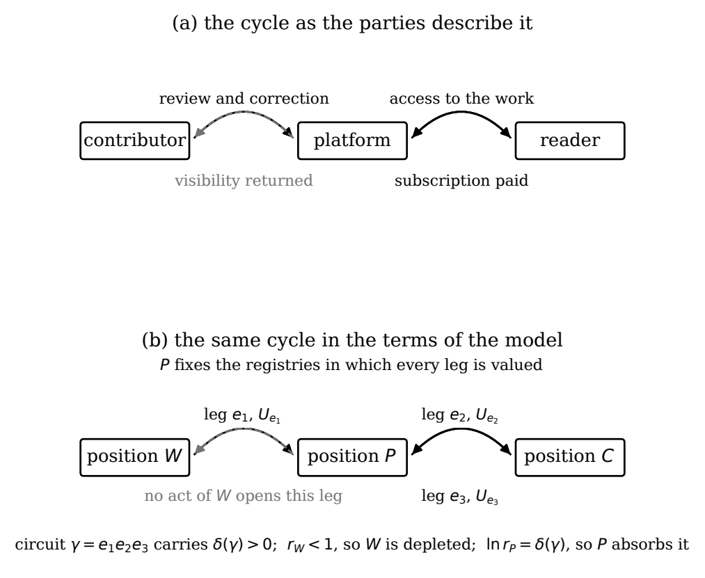
Figure 1. The objects of the model on an ordinary circulation. Panel (a) shows a cycle as the parties to it would describe it: a contributor supplies review and correction, the platform provides access to the work, the reader pays a subscription, and visibility flows back to the contributor. Panel (b) relabels the same cycle in the terms defined in this section. Each party becomes a position of Definition ?, each recurring transfer a leg carrying a transport of Definition ?, and each party’s own accounting a valuation frame of Definition ?. The dashed leg carries the condition of §11: a return that no act of the depleted party can open. The deficit, the depletion of $W$ and the absorption at $P$ are the quantities of §9 and §11, and each is stated on the circuit rather than on any leg of it.

A re-description is a map $g:V\to\Rpos$. Position $v$ replaces its registry by the rescaled registry in which every bundle receives $g_v$ times its former magnitude. A re-description is local: it is performed at a position, requires the cooperation of no other position, and asserts nothing about the world beyond $v$’s own bookkeeping.

The action of a re-description on the transports is now derived, not stipulated. Let $e=(u,v)$, and let a transfer surrender a bundle of former registered magnitude $x$ at $u$, so that by Assumption ? the former registered magnitude received at $v$ is $U_e,x$. Under the new registries, the surrendered magnitude is $x’=g_u x$ and the received magnitude is $g_v,U_e,x$. Definition ? defines the new transport as the ratio of received to surrendered registered magnitudes, so $U’_e = (g_v U_e x)/(g_u x)$, that is,

$$U’_e ;=; g_v,U_e,g_u^{-1}.$$

Equation 4 is, in its abelian form, the transformation law of a lattice gauge field, obtained here from bookkeeping alone. Two descriptions of one economy are gauge-equivalent when they differ by some $g$ in the sense of Equation 4; the physical transfers are the same, and only the registries differ.

One restriction on the identification is stated at once, since without it the construction would prove too much. If every difference of valuation were gauge, valuation would be inert, and the interpretive constitution of the economic, which this framework asserts elsewhere and does not retract, would be trivialised. The restriction is the one this series has already fixed for interpretation in general: two frames are redundantly different, and hence gauge-related, when they license the same acts; frames licensing different acts are a degree of freedom of the system and not a choice of description. Everything below quantifies over the redundant differences only, and the falsifiable direction is preserved: a single act available under one frame and not the other establishes that the difference is substantive.

5. Invariance under re-description

Let $e=(u,v)$ with $u\neq v$, and let $c\in\Rpos$ be arbitrary. There is a re-description $g$ with $U’_e=c$.

Set $g_v=c,U_e^{-1}$ and $g_w=1$ for every $w\neq v$. By Equation 4, $U’_e=g_v U_e g_u^{-1}=(c,U_e^{-1}),U_e\cdot 1=c$.

Two remarks bound the proposition. First, the re-description constructed in the proof rescales every leg incident to $v$, not the designated leg alone; the claim is only that the value of one designated leg is unconstrained, not that legs can be re-valued independently of one another. Second, two parallel legs with the same tail $u$ and head $v$ are rescaled by the same factor $g_v g_u^{-1}$, so the ratio of their transports is untouched; this is no exception to the proposition but a first instance of its complement, since the two legs together form a closed walk, out along one and back along the other, so that ratios of parallel legs are loop quantities in the sense now to be defined.

Proposition ? reaches every leg-level valuation at once. The worth of a single contribution, the amount transported by the leg from the worker to the product, the share of the consumer’s payment carried by the intermediary’s service leg: each of these can be assigned any positive value by an admissible change of registry at one endpoint. Every audit of a single transaction is an audit of a gauge-dependent quantity, and the flexibility that lawyers and accountants exploit in such audits follows from the geometry of the situation, with no bad faith required to explain it. At a point, the attribution question has no determinate answer to be found. Figure 2 shows the situation that the rest of this section makes precise.

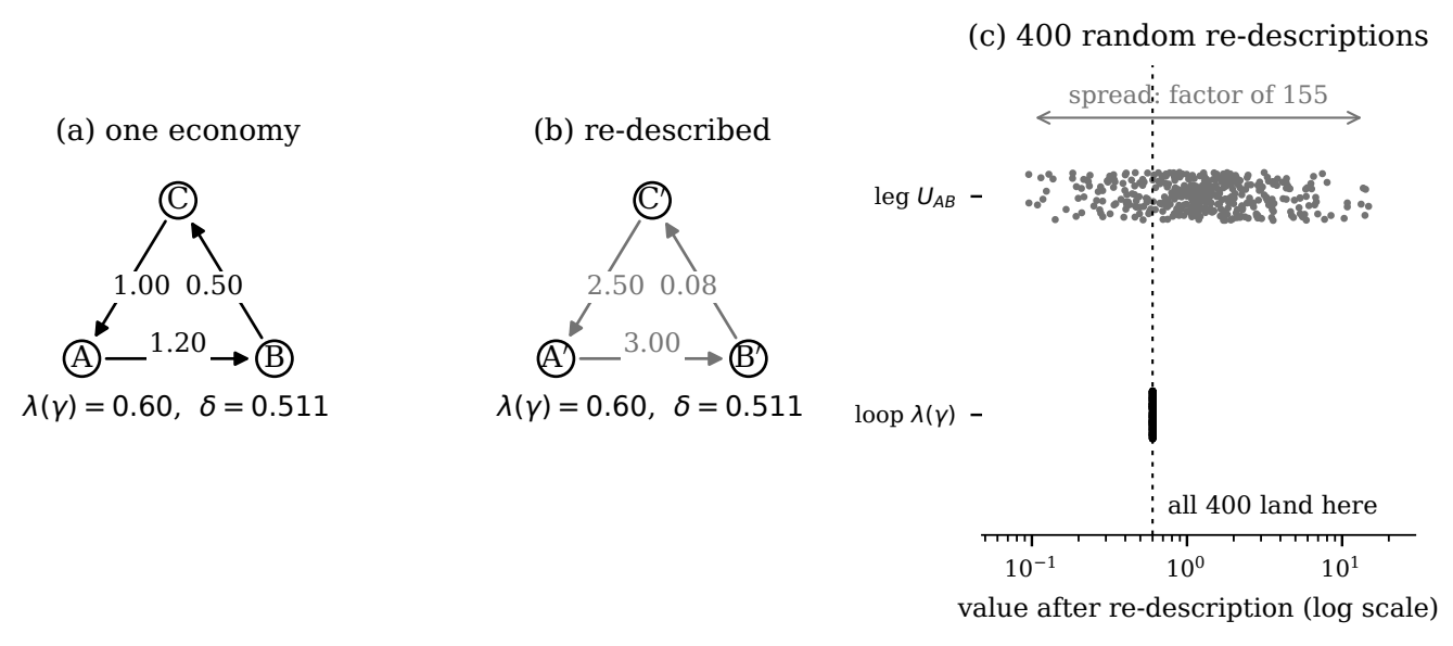
Figure 2. A re-description moves the legs and leaves the circuit alone. Panels (a) and (b) show one economy in two descriptions, related by the rescalings $g_A=1$, $g_B=2.5$, $g_C=0.4$ of Equation 4: every leg value differs, and the return ratio of the loop is $0.60$ in both. Panel (c) applies $400$ re-descriptions drawn at random and plots, on one logarithmic scale, the resulting value of the leg $A\to B$ above the resulting holonomy of the loop. The leg smears across a factor of $155$. The $400$ holonomies fall on a single mark, varying by at most $2.2\times 10^{-16}$, which is the arithmetic of the machine and not a movement. The contrast is the content of Proposition ? and Lemma ?.

For a closed walk $\gamma=(v_0,e_1,v_1,\dots,e_n,v_n{=}v_0)$ with traversal signs $\varepsilon_i$ as in Equation 3, the holonomy of $\gamma$ is

$$\hol(\gamma);=;\prod_{i=1}^{n}U_{e_i}^{\varepsilon_i},$$

the registered value returned to the starting position per unit sent around the circuit.

The holonomy of every closed walk is invariant under every re-description.

Consider a single traversed leg of $\gamma$. If $e_i$ is traversed forward, Equation 4 gives the new factor $g_{v_i}U_{e_i}g_{v_{i-1}}^{-1}$. If $e_i$ is traversed backward, the new factor is the inverse of the new forward transport, $\big(g_{v_{i-1}}U_{e_i}g_{v_i}^{-1}\big)^{-1}=g_{v_i}U_{e_i}^{-1}g_{v_{i-1}}^{-1}$. In both cases the new factor is $g_{v_i},U_{e_i}^{\varepsilon_i},g_{v_{i-1}}^{-1}$. Multiplying along the walk and using the abelian property of §6.2 to collect terms,

$$\hol’(\gamma);=;\prod_{i=1}^n g_{v_i},U_{e_i}^{\varepsilon_i},g_{v_{i-1}}^{-1}
;=;\Big(\prod_{i=1}^n U_{e_i}^{\varepsilon_i}\Big)\cdot\prod_{i=1}^n \frac{g_{v_i}}{g_{v_{i-1}}}
;=;\hol(\gamma)\cdot\frac{g_{v_n}}{g_{v_0}};=;\hol(\gamma),$$

where the middle product telescopes because each $g_{v_i}$ appears once in a numerator, from leg $i$, and once in a denominator, from leg $i{+}1$, leaving only the quotient $g_{v_n}/g_{v_0}$, which equals $1$ because $v_n=v_0$. Equation 6 is the claimed invariance.

Lemma ? states that whatever any position does to its own books, the return ratio of every closed circuit is untouched. The next theorem states the converse: the holonomies are not merely invariant, they are everything that is invariant.

Let $\Gamma$ be connected, let $T$ be a spanning tree rooted at $r$, and for each chord $e\notin T$ let $\gamma_e$ be its fundamental cycle as defined in §6.1. Then:

• (Tree gauge) There is a re-description under which $U’_e=1$ for every $e\in T$, and this re-description is unique once $g_r=1$ is fixed.
• In tree gauge, every chord carries exactly the holonomy of its fundamental cycle: $U’_e=\hol(\gamma_e)$.
• Two transport assignments are gauge-equivalent if and only if they agree on the holonomy of every closed walk; and every gauge-invariant function of the transports is a function of the fundamental holonomies ${\hol(\gamma_e):e\notin T}$ alone. The space of economies modulo description is therefore parametrised by $\Rpos^{,|E|-|V|+1}$, one coordinate per independent loop, with the exponent given by Equation 1.

(i) For each vertex $v$, let $P_v\in\Rpos$ be the composite transport, in the sense of Equation 3, along the tree path from $r$ to $v$; the tree path is unique (§6.1), so $P_v$ is well defined, and $P_r=1$ as an empty product. Define

$$g_v ;=; P_v^{-1},$$

so that $g_r=1$. Let $e=(u,v)$ be a tree edge. Removing $e$ from the tree separates the vertices into two components, and the root lies in exactly one of them. If $r$ lies on the tail side, the tree path to $v$ is the tree path to $u$ followed by $e$ forward, so $P_v=U_e P_u$ by Equation 3, and Equation 4 with Equation 7 gives $U’_e=P_v^{-1}U_eP_u=(U_eP_u)^{-1}U_eP_u=1$. If $r$ lies on the head side, the tree path to $u$ is the tree path to $v$ followed by $e$ backward, so $P_u=U_e^{-1}P_v$, and $U’_e=P_v^{-1}U_e(U_e^{-1}P_v)=1$. For uniqueness, suppose $g$ and $h$ both satisfy $g_r=h_r=1$ and put every tree transport at $1$. Then along every tree edge $e=(u,v)$, both $g_vU_eg_u^{-1}=1$ and $h_vU_eh_u^{-1}=1$, so $g_v/g_u=h_v/h_u$; the ratio $g_v/h_v$ is therefore constant across every tree edge, and since the tree connects all vertices and $g_r/h_r=1$, the ratio is $1$ everywhere.

(ii) For a chord $e=(u,v)$, Equations 4 and 7 give $U’_e=P_v^{-1}U_eP_u$. The right-hand side is, by Equation 3, the product of transports along the walk that goes from $r$ to $u$ along the tree, contributing $P_u$, crosses $e$ forward, contributing $U_e$, and returns from $v$ to $r$ along the tree reversed, contributing $P_v^{-1}$. That walk is the fundamental cycle $\gamma_e$, so $U’_e=\hol(\gamma_e)$ by Equation 5.

(iii) The forward direction is Lemma ?: gauge-equivalent assignments share every holonomy. For the converse and the classification, first observe that in tree gauge the holonomy of any closed walk $\gamma$ reduces to a product over the chords it uses. Tree legs contribute the factor $1$ in tree gauge, so by Equation 5,

$$\hol(\gamma);=;\prod_{e\notin T}\hol(\gamma_e)^{,n_e(\gamma)},$$

where $n_e(\gamma)$ is the net signed number of times $\gamma$ traverses the chord $e$, that is, forward traversals minus backward traversals, and Equation 8 uses part (ii) to write each chord’s tree-gauge transport as a fundamental holonomy. Since holonomies are gauge-invariant by Lemma ?, Equation 8 holds in every gauge, not only in tree gauge. Now suppose two assignments $U$ and $\widetilde U$ share every holonomy. Place each in its tree gauge; by part (ii) the resulting normal forms are determined entirely by the fundamental holonomies, which agree, so the normal forms are identical, and the two assignments, being each gauge-equivalent to a common assignment, are gauge-equivalent to one another. Finally, let $F$ be any gauge-invariant function of the transports. $F$ is constant on each gauge orbit. Each orbit contains exactly one assignment in tree form: existence is part (i); and if two tree-form assignments lay in one orbit, the re-description $h$ relating them would satisfy $h_vh_u^{-1}=1$ across every tree edge by Equation 4, hence would be constant on the connected tree, and a constant re-description fixes every transport, so the two assignments coincide. By part (ii) that unique representative is the list of fundamental holonomies together with $1$’s on the tree. Hence $F$ factors through the vector $\big(\hol(\gamma_e)\big)_{e\notin T}$, which has $|E|-|V|+1$ components by Equation 1, each ranging freely over $\Rpos$.

Theorem ? is the formal statement of a claim this framework has made in responsibility and in governance and now makes in economics: the difficulty of point attribution is a symptom, and the question itself is misdirected; the content that can be objectively stated about a transfer structure is carried by its loops. The dimension count states the same thing numerically. A network with $|E|$ legs supports $|E|$ leg-level accounting disputes, of which exactly $|E|-|V|+1$ dimensions survive re-description, and those dimensions are indexed by circuits, not by transactions. Figure 3 displays the normal form the proof constructs.

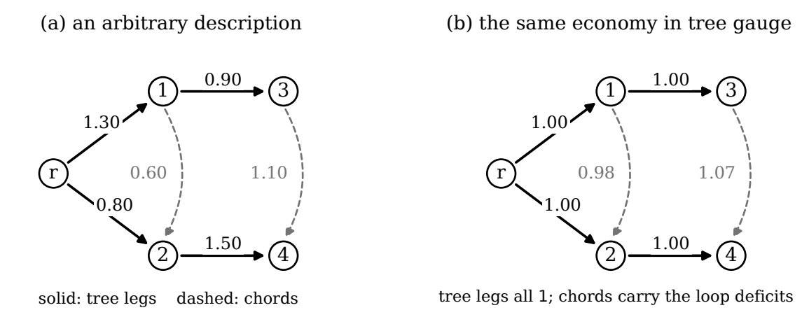
Figure 3. The tree gauge of Theorem ?. The network has five positions and six legs, so its cycle rank is $6-5+1=2$ by Equation 1. Panel (a) is an arbitrary description. Panel (b) is the same economy after the re-description of Equation 7: every tree leg now transports exactly $1$, and each chord carries the holonomy of its fundamental cycle, here $0.975$ and $1.0725$. Six accounting numbers have become two, and the two are the loops.

6. The loop deficit and the obstruction to a global measure of value

For a closed walk $\gamma$, the loop deficit is

$$\delta(\gamma);=;-\ln\hol(\gamma).$$

By the properties of the logarithm collected in §6.2: $\delta(\gamma)=0$ states that the circuit closes, a unit sent around $\gamma$ returning as a unit; $\delta(\gamma)>0$ states that the circuit returns less than was sent, which is a deficit; and $\delta(\gamma)<0$ states that it returns more, which is a surplus.

Three properties follow directly. By Lemma ? and Equation 9, $\delta$ is invariant under every re-description. Reversing the orientation of $\gamma$ inverts every factor of Equation 5 and so reverses the sign, $\delta(\gamma^{-1})=-\delta(\gamma)$. For two loops $\gamma_1,\gamma_2$ sharing a basepoint and traversed one after the other as the concatenation $\gamma_1\cdot\gamma_2$, the holonomies multiply, so the deficits add:

$$\delta(\gamma_1\cdot\gamma_2);=;\delta(\gamma_1)+\delta(\gamma_2).$$

The deficit compares the same bundle at the same position before and after one circuit. It is a ratio at a point, so it requires no common unit across kinds of value, no cardinal measure of generativity, and no comparison between persons. In particular the uniform re-descriptions $g_v=c$ for all $v$, which constitute a global change of unit, leave every transport unchanged by Equation 4 and every deficit unchanged exactly. This is what permits the framework to possess an assessable quantity while maintaining that generativity itself has no unit and cannot be maximised: the deficit is defined per loop, and neither Equation 9 nor Equation 10 licenses summing deficits across distinct loops of different basepoints, or across persons. Deficits of distinct loops are accordingly not commensurable, and no aggregate deficit of an economy is defined by this construction.

The deficit now receives its structural role: it stands between a transfer network and a global measure of value.

Write $a_e=\ln U_e$ for each leg. Say that $\varphi:V\to\mathbb{R}$ is a value potential if

$$a_e;=;\varphi(v)-\varphi(u)\qquad\text{for every leg }e=(u,v),$$

that is, a level of value assignable to every position, of which every leg’s logarithmic rate is the difference. Then a value potential exists if and only if $\delta(\gamma)=0$ for every closed walk $\gamma$; and where it exists it is unique up to one additive constant.

Write, for any walk $p$ with traversal signs $\varepsilon_i$, the signed sum $\sigma(p)=\sum_i \varepsilon_i a_{e_i}$; by Equations 5 and 9 and the product-to-sum property of $\ln$, a closed walk satisfies $\sigma(\gamma)=\ln\hol(\gamma)=-\delta(\gamma)$.

Necessity. Suppose Equation 11 holds. Along any walk, each term of $\sigma$ is $\varepsilon_i,(\varphi(\text{head})-\varphi(\text{tail}))=\varphi(v_i)-\varphi(v_{i-1})$, whether the leg is traversed forward or backward, so the sum telescopes: $\sigma(p)=\varphi(v_n)-\varphi(v_0)$. For a closed walk $v_n=v_0$, hence $\sigma(\gamma)=0$, hence $\delta(\gamma)=0$.

Sufficiency. Suppose every closed walk has zero deficit. Fix a basepoint $r$ and define $\varphi(v)=\sigma(p)$ for any walk $p$ from $r$ to $v$; connectivity supplies such a walk. Well-definedness: if $p$ and $q$ are two walks from $r$ to $v$, then $p$ followed by $q$ reversed is a closed walk, and $\sigma(p)-\sigma(q)=\sigma(p\cdot q^{-1})=-\delta(p\cdot q^{-1})=0$ by hypothesis. Equation 11: for a leg $e=(u,v)$, extend a walk from $r$ to $u$ by the single forward step $e$; the definition of $\varphi$ gives $\varphi(v)=\varphi(u)+a_e$.

Uniqueness. If $\varphi$ and $\psi$ both satisfy Equation 11, their difference has zero difference across every leg, and a function on a connected graph with zero difference across every leg is constant.

Theorem ? converts a familiar demand into a question with a determinate answer. A global measure of value is a single scale on which every position’s holdings could be consistently stated, so that every transfer is a mere movement along the scale. Such a measure is exactly a potential in the sense of Equation 11, and the theorem states when one exists: precisely when every loop closes. The two directions carry different lessons. Where deficits exist, there is no global measure, and any party using one has imposed it; the imposition may be necessary or best, but it is an act performed at a position and not a discovery. Where a global measure exists, every circuit closes identically, and there is nothing invariant left for the measure to detect beyond its own level differences. A maximand is a potential; recommending one therefore presupposes the vanishing of exactly the quantity this paper identifies as the frame-independent content of circulation. Maximisation is available only where there is nothing to find.

Figure 4 draws a deficit, and then draws the refinement that locates it, using the case worked in §12.

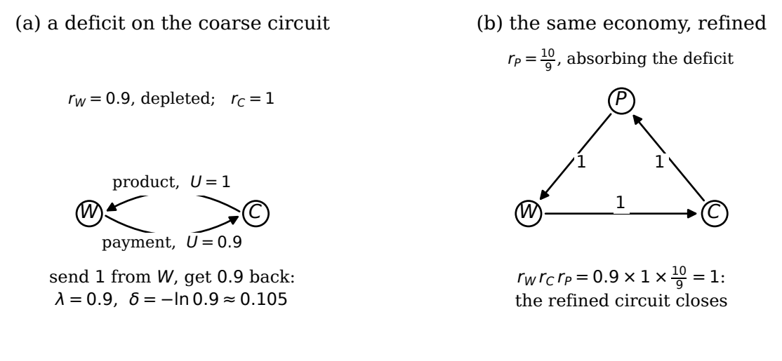
Figure 4. A loop deficit, and the position it names. In panel (a) a unit sent from $W$ around the circuit returns as $0.9$, so $\delta=-\ln 0.9\approx 0.105$, and by Lemma ? it sits entirely at $W$, whose retention ratio is $0.9$. Panel (b) refines the network by the intermediary $P$ in the sense of Definition ?: the original retention ratios are unchanged, $P$ retains $10/9$, and the refined circuit closes, since $0.9\times 1\times 10/9=1$. A deficit on a coarse circuit is the registered retention of a position the description omitted.

7. The correspondence

Table 1 states the concept mapping in full, each row resting on a definition or result already given. The last three rows record deliberate absences: concepts of the source theory to which the paper assigns no economic counterpart and from which it takes nothing.

| @ll@

Gauge theory	Economy of transfers
base space	transfer network $\Gamma$ (Def. ?)
fibre over a point	valuation registry at a position (Def. ?)
gauge transformation	re-description of a position’s accounting (Def. ?, Eq. 4)
connection / parallel transport	terms of exchange on a leg (Def. ?, Eq. 3)
gauge-dependent quantity	worth of a single leg or contribution (Prop. ?)
holonomy of a loop	return ratio of a closed circuit (Def. ?, Lem. ?)
curvature (plaquette holonomy)	loop deficit on a fundamental cycle (Def. ?; see note)
matter field on a site	capacity stock at a position (Counterexample ?)
flat connection	circulation closing on every circuit
existence of a potential	consistent global measure of value (Thm. ?)
gauge fixing (tree gauge)	an imposed standard accounting (Thm. ?(i))
dynamics, action, Lagrangian	no counterpart taken
physical constants and scales	no counterpart taken
continuum limit	no counterpart taken

Table. The concept mapping. Every row above the lower rule is definitional within this paper; the rows below it name the concepts the borrowing excludes.

Four rows require comment. Each row of the table asserts a correspondence, and each such assertion is checked below against the definition or result it cites.

The tree-gauge row gives the formal position of standard accounting: a uniform frame can always be imposed, since Theorem ?(i) constructs one; it simplifies every book; and it constitutes a choice made at a position rather than a neutral fact, while everything invariant, being carried by the chords, is unchanged by the imposition and remains computable by anyone who knows what was imposed. One reassurance belongs here: on a connected graph the tree gauge exists globally and without obstruction, so the well-known difficulties of gauge fixing in continuum theories play no role in this paper, and the mapping does not lean on unsettled physics at this point.

The curvature row is looser than the others. In lattice gauge theory, curvature is the holonomy of a minimal two-dimensional cell, a plaquette, and a bare graph possesses no two-dimensional cells; what exists on a graph is holonomy, and once a spanning tree is chosen the fundamental cycles play the role the plaquettes play on a lattice. The paper accordingly treats “deficit” as its exact term and “curvature” as the informal name of the analogy; every result in the paper is stated and proved for holonomies and deficits, and nothing depends on the looser word.

The potential row can be sharpened into an equivalence. Substituting $g_v=e^{-\varphi(v)}$ into Equation 4 shows that Equation 11 holds exactly when the transports are gauge-equivalent to the trivial assignment $U_e=1$ on every leg. Zero deficit therefore says something stronger than “the books balance”: it says the entire economy is a re-description of an economy in which no conversion occurs at all, and bookkeeping alone neither produces nor removes a non-zero deficit.

The matter row explains, structurally, a result proved in §11: in lattice terms the transports live on links and the capacity stocks of Counterexample ? live on sites; the deficit is an observable of the link sector alone, and the wrong exhibited by that counterexample lives in the site sector, which is the geometric reason the deficit leaves it unregistered. Finally, the curvature row is the paper’s title, and §11 determines how much normative weight it carries: less than the title suggests, and as much as the conditions stated there.

8. Deficit and exploitation: the mapping is strict in both directions

The intuition to be examined is that a non-zero deficit is the footprint of extraction: value was drained from the circuit even though every leg looked fair, and the loop registers what the legs conceal. The intuition holds in one direction and fails in the other, and a framework built on the equation would inherit the failure. The deficit is an observable and not a criterion. Both failures of the equation between deficit and exploitation are now exhibited, and the joint conditions that the failures force are then stated with every term defined.

Let $\Gamma$ have two positions, a producer $W$ and a household $H$, with a product leg $W\to H$ of transport $1$ and a payment leg $H\to W$ of transport $0.8$: the household returns four fifths of the registered value and consumes the rest, finally, as use. The unique loop $\gamma$ has, by Equations 5 and 9,

$$\hol(\gamma)=1\times 0.8=0.8,\qquad \delta(\gamma)=-\ln 0.8\approx 0.223>0.$$

Nothing in the situation is a wrong; final consumption is the point of the circuit, not a leak in it. The same structure is exhibited by a consented subsidy, in which a mentor, patron or commons knowingly returns less than it receives, and by depreciation. An economy in which every loop closed would be an economy in which nothing was ever finally used. A criterion condemning the positive deficit of Equation 12 condemns eating.

Let $\Gamma$ be any cycle with every transport equal to $1$, so that $\delta(\gamma)=0$ on every closed walk by Equation 9: the flow account closes exactly, period after period. Separately from the flow account, let $k(t)\in\Rpos^{V}$ record the stock of capacity held at each position after $t$ periods, and let one period of the closed circulation redistribute stocks linearly,

$$k(t{+}1);=;M,k(t),$$

with $M$ column-stochastic in the sense of §6.4; by Equation 2 the total stock is conserved at every step, which is the stock-level counterpart of loop closure. Take two positions and

$$M=\begin{pmatrix}0.9&0.6\[2pt]0.1&0.4\end{pmatrix},\qquad k(0)=\begin{pmatrix}1\[2pt]1\end{pmatrix}.$$

The behaviour of Equation 13 is computed from scratch. The eigenvalues of $M$ solve $\det(M-\mu I)=\mu^2-1.3\mu+0.3=(\mu-1)(\mu-0.3)=0$, so they are $\mu_1=1$ and $\mu_2=0.3$. An eigenvector for $\mu_1=1$ solves $-0.1,x+0.6,y=0$, giving $x=6y$; normalised to the conserved total $2$, the eigenvector is $\pi=(12/7,,2/7)^{\mathsf T}$. An eigenvector for $\mu_2=0.3$ solves $0.6,x+0.6,y=0$, giving $w=(1,-1)^{\mathsf T}$. Writing the initial stock in this basis, $k(0)=\pi+c,w$ requires $12/7+c=1$, so $c=-5/7$, and applying Equation 13 $t$ times multiplies each component by its eigenvalue:

$$k(t);=;\pi;-;\tfrac{5}{7},(0.3)^{t},w;\longrightarrow;\pi=\begin{pmatrix}12/7\[2pt]2/7\end{pmatrix}\quad\text{as }t\to\infty .$$

Equation 15 exhibits the wrong: the total is conserved at every step, the deficit is identically zero, and capacity concentrates at the first position while the second is run down to one seventh of the total and becomes dependent on the first for every subsequent period. The concentration is monotone in $t$, structural, and entirely invisible to $\delta$, because $\delta$ is a flow observable and the wrong is a stock phenomenon; in the vocabulary of Table 1, the transports are link variables, the stocks are site variables, and the deficit is an observable of the link sector alone. Coupled loops exhibit the same failure one level up: a measured financial loop may close exactly while the unmeasured relational loop that sustains it is depleted.

No function of $\delta$ alone is a criterion of exploitation.

Suppose $f$ maps deficit values to verdicts. Counterexample ? exhibits a benign circuit of deficit $-\ln 0.8$; a circuit satisfying Conditions ?, ? and ? below can be constructed with the same numerical deficit (take the worked case of §12 with its payment transport set to $0.8$), so $f$ returns one verdict on a benign and an extractive economy of equal $\delta$. Counterexample ? and a fully benign closed loop share the value $\delta=0$, so $f$ fails again in the other direction. In each direction $f$ fails to separate the classes it was to separate.

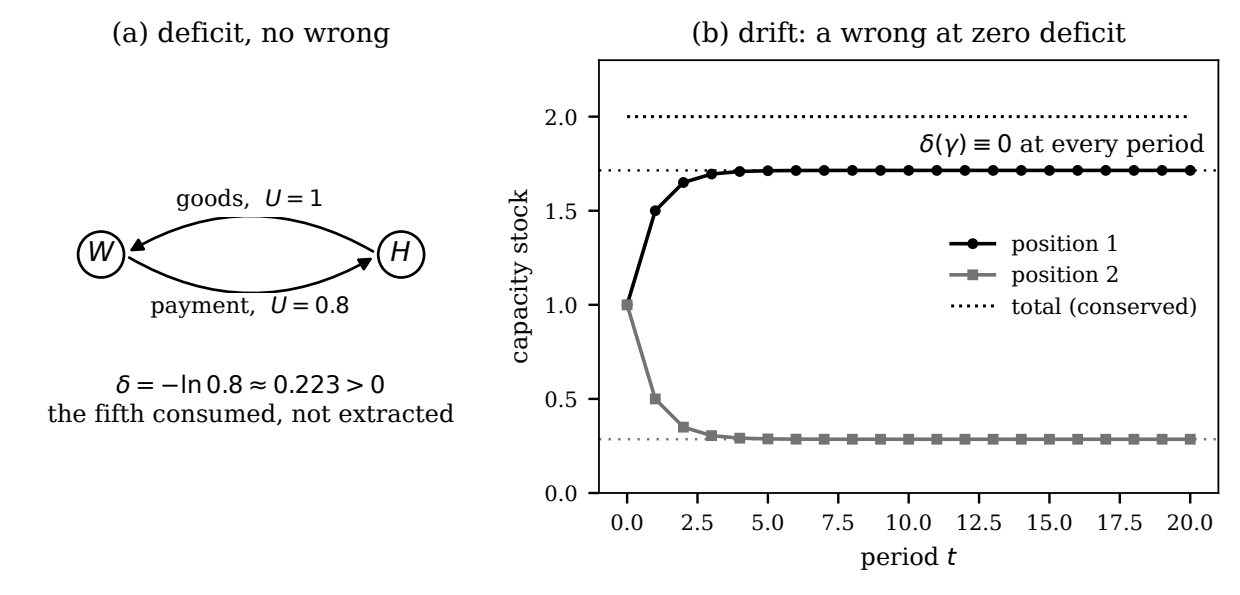
Figure 5. The two directions in which deficit and exploitation come apart. Panel (a) is Counterexample ?: the household returns four fifths and consumes the rest, so $\delta\approx 0.223>0$ with nothing extracted from anyone. Panel (b) is Counterexample ?, simulated for twenty periods from Equations 13 and 14: the total stock is conserved to ten decimal places and every circuit closes, so $\delta\equiv 0$, while capacity concentrates monotonically at the first position and converges to the values $12/7$ and $2/7$ computed in closed form at Equation 15. A criterion reading exploitation off the deficit alone would acquit panel (b) and convict panel (a).

Corollary ? fixes the sense in which the title’s phrase “measures of structural exploitation” can be maintained: the deficit measures, in the sense of an instrument, invariantly and without a unit, while it does not judge. What it is an instrument for is stated by joint conditions, and stating them requires two prior definitions, since “depleted” and “absorbing” carry weight in what follows. Both definitions rest on a decomposition of the deficit into position-level quantities, which is proved first.

Let $\gamma$ be a cycle through positions $v_0,v_1,\dots,v_{n-1}$ in order, with leg $e_i$ running from $v_{i-1}$ to $v_i$, all indices taken modulo $n$. Suppose the circuit operates in steady flow: in each period, position $v_i$ surrenders a bundle of registered magnitude $x_i$ along $e_{i+1}$ and receives, by Assumption ?, registered magnitude $y_i=U_{e_i}x_{i-1}$ along $e_i$, with the same magnitudes every period. Define the retention ratio of position $v_i$ as $r_i=y_i/x_i$, the registered magnitude received per registered magnitude surrendered, both in $v_i$’s own frame. Then each $r_i$ is invariant under every re-description, and

$$\prod_{i=0}^{n-1} r_i;=;\hol(\gamma),
\qquad\text{equivalently}\qquad
\sum_{i=0}^{n-1}\big(-\ln r_i\big);=;\delta(\gamma).$$

Invariance of $r_i$: a re-description rescales both $y_i$ and $x_i$ by the same factor $g_{v_i}$, since both are magnitudes in $v_i$’s registry, and the ratio cancels the factor. For Equation 16: substituting $y_i=U_{e_i}x_{i-1}$,

$$\prod_{i=0}^{n-1} r_i;=;\prod_{i=0}^{n-1}\frac{U_{e_i},x_{i-1}}{x_i}
;=;\Big(\prod_{i=0}^{n-1}U_{e_i}\Big)\cdot\frac{\prod_{i}x_{i-1}}{\prod_{i}x_i}
;=;\hol(\gamma),$$

since the indices run over the same cyclic set, making the quotient of the two $x$-products equal to $1$, and the product of the transports is $\hol(\gamma)$ by Equation 5. Taking $-\ln$ of Equation 17 and using the product-to-sum property gives the additive form, by Equation 9.

Lemma ? distributes the loop deficit exactly over the positions on the loop: each position’s net gain or loss, measured in its own registry and invariant under all re-description, contributes $-\ln r_i$ to the total, and the contributions sum to $\delta(\gamma)$ by Equation 16. The two required definitions follow.

A position $v_i$ on a steadily operating cycle $\gamma$ is depleted when $r_i<1$ persistently, that is, in every period: the position surrenders more registered value than it receives, period after period, in its own frame. By Lemma ? the property is invariant under re-description.

Let $\gamma$ carry a deficit $\delta(\gamma)>0$ in a network $\Gamma$. A position $b$ absorbs the deficit when there is a refinement of $\Gamma$, obtained by adding $b$ and rerouting one or more legs of $\gamma$ through $b$ (replacing a leg $(u,w)$ by legs $(u,b)$ and $(b,w)$), under whose steady flow every original position on $\gamma$ retains the retention ratio it had before, while $b$’s retention ratio satisfies $\ln r_b=\delta(\gamma)$: the value missing from the circuit reappears, exactly, as $b$’s registered net gain.

The conditions can now be stated. They are stated per depleted position; no aggregation across persons enters, and no surplus of health elsewhere in the network offsets a failure at one position.

There is a loop $\gamma$ with $\delta(\gamma)>0$ in every period over which it recurs, and an identifiable position $b$ that absorbs it in the sense of Definition ?.

The absorbing position $b$ controls the description of the network itself: it fixes the frames in which legs are valued, or fixes which transfers are recorded as legs of $\Gamma$ at all. The party into whose registry the deficit closes is the party that draws the map on which the deficit would be sought.

No act available to a depleted position, in the sense of Definition ?, establishes or re-opens a leg toward that position whose inclusion would raise its retention ratio to $1$; and the performance of such acts as are available places $b$ under no obligation to answer. The initiative that would repair the circuit does not lie with the position the circuit depletes.

Jointly, Conditions ?, ? and ? characterise structural exploitation as this framework can state it: a persistent deficit, absorbed at a position that controls the accounting, which the depleted position holds no available act to close. Each condition is structural and present-tense; none is a forecast, and none aggregates. Counterexample ? fails Condition ?, since the household’s retention is the producer’s own purpose in the circuit, or is open to renegotiation at the producer’s instance; this is why consumption is no wrong. Counterexample ? fails Condition ?, since there is no deficit to absorb; this is why drift requires its own detection on stock histories such as Equation 15 and panel (b) of Figure 5, as a fourth structure the deficit cannot supply, and why circulation criteria, this paper’s included, are necessary and not sufficient.

9. Localisation, the worked case, and the observer

What, then, does the invariance of the deficit contribute, if the deficit does not itself convict? The answer is the paper’s principal claim.

Let two parties agree on the network $\Gamma$ and on the transports as matters of fact. Then they agree on every deficit, whatever frames either adopts and however either re-describes any leg. Contrapositively: a disagreement about a deficit that persists is a disagreement about $\Gamma$, that is, about whether a leg exists and carries a genuine transport, or about a transport’s factual value; it is never a disagreement of description.

Immediate from Theorem ?(iii): the deficits are functions of the gauge orbit, and the orbit is fixed by the factual data $(\Gamma, U)$.

The proposition removes the force of one class of defences and localises the remainder. The class that loses its purchase is the defence that operates by re-describing transactions, of the form “under our accounting, each step was fair”: by Proposition ? such re-descriptions can set a designated leg to an arbitrary value, and by Lemma ? they leave every deficit unchanged. The localised remainder is a factual dispute about the graph. The worked case makes the mechanics explicit.

The intermediary’s fee. A creator $W$ supplies work valued at $100$ to a consumer $C$ through a platform $P$; the consumer pays $100$; the creator receives $90$. On the network $\Gamma_1$ with positions ${W,C}$ and the two legs $W\to C$ of transport $1$ and $C\to W$ of transport $0.9$, the loop carries

$$\delta;=;-\ln 0.9;\approx;0.105,$$

and by Lemma ? the quantity in Equation 18 sits entirely at $W$: the retention ratios are $r_W=0.9$ and $r_C=1$, so $W$ is depleted in the sense of Definition ? and $C$ breaks even. Three observations. First, the raw computation “paid $100$, received $90$” is a flow imbalance within one description, and standing alone it is exactly the kind of leg-level, gauge-dependent claim that Proposition ? empties; the invariant content appears only when the claim is stated on the closed circuit, as the deficit of Equation 18, which no re-registration at $W$, $C$, or anywhere else can alter. Second, the platform’s standard defence, that the ten is the price of a real service such as matching, hosting or trust, is not a re-description. It is a proposal to change the graph: to adopt a refinement $\Gamma_2$ in which $P$ is a position, the payment routes $C\to P\to W$, and a further leg $P\to W$ carries the service. Definition ? separates the two things the defence asserts. Rerouting the payment as $C\to P$ and $P\to W$, each leg at transport $1$, with $P$ receiving the registered $100$ and surrendering $90$, leaves the original retention ratios $r_W=0.9$ and $r_C=1$ unchanged and gives $\ln r_P=\ln(10/9)=\delta$, which establishes exactly that $P$ absorbs the deficit in the sense of Definition ?, satisfying Condition ?. Equation 16 has a further consequence here. In the refined graph the circuit through $P$ satisfies $r_W,r_C,r_P=0.9\times 1\times(10/9)=1$ and therefore closes, so the deficit of the coarse circuit $\Gamma_1$ is the registered retention of the position its description omitted. A deficit names an absentee. The further service leg, if its transport is genuine, would raise $r_W$ to $1$ and close $W$’s own account. Third, the choice between the graphs is not a choice of frame, and Proposition ? says no choice of frame can ever settle or unsettle it. Whether the service leg carries a genuine transport, that is, whether what $P$ provides in fact enters $W$’s capacity to re-create what $W$ contributes, is a factual question about the world, checkable in principle, and the entire dispute about the fee has been moved onto it. That movement is the contribution: the loop observable does not answer the question of exploitation, it moves the question into a form in which accounting ingenuity has little purchase and evidence becomes relevant. Conditions ?, ? and ? then state the burden for the evidence.

One consequence of the construction tells against it. Computing $\delta(\gamma)$ requires, by Equation 5, the transports of every leg on $\gamma$; a party occupying one position holds one leg. In the platform case the only party that holds the complete circuit record, that is, who transferred what to whom, at what registered rates, around the whole loop, is ordinarily the intermediary itself. The invariant that would detect extraction is therefore computable, in practice, only by the party best positioned to extract. The paper draws the minimal consequence rather than a policy programme: disclosure of circuit-level records is not one transparency measure among others but the condition of possibility for anyone other than the intermediary to use the observable defined here, and an intermediary declining such disclosure has not merely withheld data; it has reserved to itself the only standpoint from which the invariant content of its own economy can be seen.

10. Further discussion: heterogeneous value, phase, and loop homology

Everything above treats value as one kind: the fibre is a single magnitude, and a transport is a single ratio. Value is heterogeneous, being financial, epistemic, relational and infrastructural at least, and the question this section opens, without settling, is how far the loop framework extends to that heterogeneity. Two extensions are sound and cheap, and this paper claims them; the honest general treatment is neither, and is deferred.

The cheapest extension attaches a phase to each transport, taking the transports in the multiplicative group of non-zero complex numbers:

$$U_e;=;\rho_e,e^{i\theta_e},\qquad \rho_e\in\Rpos,\quad \theta_e\in(-\pi,\pi],$$

where the modulus $\rho_e$ is the conversion ratio as before and the angle $\theta_e$ is offered as a coordinate on the kind of conversion the leg performs. The group of Equation 19 is abelian, so Lemma ? holds verbatim, and every closed walk now carries an invariant pair: the modulus deficit already defined, and a phase holonomy,

$$\delta(\gamma);=;-\sum_i \varepsilon_i \ln\rho_{e_i},
\qquad
\Theta(\gamma);=;\sum_i \varepsilon_i,\theta_{e_i}\ \ (\mathrm{mod}\ 2\pi),$$

each invariant under every re-description by the same telescoping argument. The pair of Equation 20 can register a situation the scalar theory cannot: $\delta(\gamma)=0$ with $\Theta(\gamma)\neq 0$ says the circuit returns full magnitude in a transformed kind, closure in quantity without closure in kind, which is the formal shadow of the coupled-loop concern recorded at the end of Counterexample ?, where a financial loop closes while the relational loop sustaining it does not.

The second sound extension is the classification. The proof of Theorem ? uses only the invertibility of transports and the abelian property, so it carries over unchanged to transports valued in any abelian group $G$, and its content can then be stated in the language of loop homology. The first homology group $H_1(\Gamma;\mathbb{Z})$ of a graph is the free abelian group generated by the fundamental cycles of any spanning tree, so a homomorphism out of it is fixed by its values on those cycles, and Theorem ?(iii) becomes

$${\text{economies on }\Gamma}\big/{\text{re-descriptions}};\cong;\mathrm{Hom}\big(H_1(\Gamma;\mathbb{Z}),,G\big);\cong;G^{,|E|-|V|+1}.$$

Equation 21 says in one line what the paper has argued in many: the space of economies modulo description is the space of loop-valuations, one $G$-value per independent loop, and nothing else. The scalar theory of this paper is the case $G=\Rpos$; the phase extension is $G=\Rpos\times U(1)$.

The interpretation is not yet sound, and the discipline of §5 applies to this section with full force. Under Equation 19 the composition of two legs adds their angles, so the admission test demands an economic operation to which the addition of kind-angles corresponds; kinds of value are discrete and are not, in general, arranged on a circle, so the phase reading fits only where conversions between kinds genuinely compose cyclically, and a finite cyclic group would then be the more candid choice than $U(1)$. Where kinds neither cycle nor commute, the honest object is a value space of several dimensions at each position, possibly of different dimensions at different positions, with matrix-valued transports; the group is then non-commutative, the holonomy of a loop depends on its basepoint up to conjugation, the domain of the classification is the fundamental group of the graph, a free group of rank $|E|-|V|+1$, in place of its homology, and the invariants are the conjugation-invariant functions of the holonomy, its spectrum and traces, in place of the holonomy itself. Two exclusions are recorded at the point of definition, as §5 requires: the phase of Equation 19 carries no connotation of amplitude, probability, superposition, or interference; and no claim is made that any actual system of value kinds satisfies the cyclic composition the phase reading presupposes. The two sound anchors, the invariant pair of Equation 20 and the classification of Equation 21, are claimed by this paper; the heterogeneous fibre theory, with its position-dependent value spaces and non-commuting conversions, is a separate undertaking with a different mathematical register, and is deferred to a companion treatment.

11. Limits

Six limits, in decreasing order of severity.

First, the admission test restricts the scope, and the restriction excludes hard cases. The construction requires transports that compose along paths as in Equation 3 and invert, which registered monetary and quantifiable in-kind legs satisfy to good approximation. Legs of the form labour to product, or care to capacity, do not obviously satisfy either requirement, and no claim is made that they do; loops containing such legs fall outside the model until a group structure for them is exhibited rather than assumed. Several of the deepest questions of value concern exactly those legs, so the restriction removes them from the paper’s reach.

Second, Assumption ? idealises. Actual terms of exchange include thresholds, volume discounts, and other non-linearities under which the transport is not a single ratio, and Lemma ? additionally assumes steady flow, without which retention ratios fluctuate and the statements of §11 hold per period rather than once for all. Both are idealisations, and results stated under them hold only so far as they hold.

Third, the graph is stipulated, and Proposition ? pushes the surviving disputes onto the object the paper stipulates. The localisation result therefore takes this form: the construction converts valuation disputes into topology disputes, and supplies no procedure for settling the latter. The conversion is claimed as progress, since topology disputes are factual and evidence-apt where valuation disputes are not. That claim rests on a judgement about which kind of dispute is more tractable, and a reader who judges otherwise loses the section’s conclusion while keeping its proposition.

Fourth, the gauge group is stipulated. That admissible re-descriptions compose, invert, and commute are three separate empirical claims about actual accounting practices, and the abelian choice made here is the simplest available rather than the established one. Value of several kinds, financial, epistemic, relational and infrastructural, converting in an order-dependent way would require a non-abelian group, under which Lemma ? survives with conjugation-invariant functions of the holonomy in place of the holonomy itself; the coupled-loop failures gestured at in Counterexample ? live there; §13 fixes the reach of the abelian phase extension, and the heterogeneous fibre theory is deferred to a companion treatment.

Fifth, the magnitude of a deficit is uninterpreted. The construction distinguishes zero from non-zero and orders deficits on a single loop over time; it assigns no social meaning to any particular value of Equation 9, and Corollary ? blocks the reading of a threshold as a verdict.

Sixth, the relation to the existing gauge economics is easily overstated in either direction. Ilinski’s(Ilinski, Kirill, mph Physics of Finance:, n.d.) curvature is arbitrage and prices it away in equilibrium; the present deficit is defined over valuation frames and survives arbitrage-free pricing, so the constructions are distinct. A reader persuaded that all economic curvature reduces to arbitrage will find the present object either novel or empty, a disjunction this position paper states and does not resolve.

The paper’s established claims are these. The worth of a leg is a description (Proposition ?); the deficit of a loop is a fact (Lemma ?, Theorem ?); a global measure of value exists only where every loop closes (Theorem ?); and exploitation, which the deficit evidences and cannot adjudicate (Corollary ?), is a joint structural condition of absorption, schema power, and blocked return, whose dispute the invariance of the deficit forces out of accounting and into the world (Proposition ?).

References

Eglash, Ron, “An Introduction to Generative Justice,” Teknokultura 13(2), 2016, 369–404. doi:10.5209/rev_TEKN.2016.v13.n2.52847.

Emmanuel, Arghiri, Unequal Exchange: A Study of the Imperialism of Trade, translated by Brian Pearce, Monthly Review Press, 1972. French original L’échange inégal, François Maspero, 1969.

Ilinski, Kirill, Physics of Finance: Gauge Modelling in Non-Equilibrium Pricing, Wiley, 2001.

Malaney, Pia, The Index Number Problem: A Differential Geometric Approach, PhD dissertation, Harvard University, 1996.

Marx, Karl, Capital: A Critique of Political Economy, Volume II: The Process of Circulation of Capital, 1885.

Young, K., “Foreign exchange market as a lattice gauge theory,” American Journal of Physics 67(10), 1999, 862–868.

Sraffa, Piero, Production of Commodities by Means of Commodities: Prelude to a Critique of Economic Theory, Cambridge University Press, 1960. thebibliography